1. Motivating example
Let’s start with a motivating example, without yet justifying why we are doing these steps. We will create a generative model for sampling from the uniform distribution over \(\{+1, -1\}\), i.e., a signed Bernoulli random variable. To do so requires two parts: training, and sampling.
Training
Training involve sampling from the data distribution
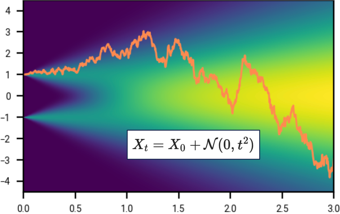
\[\begin{equation} \label{eq:signed_bernoulli_distribution} X_0 \sim \begin{cases} +1 ~\text{ with probability } 1/2, \\ -1 ~\text{ with probability } 1/2. \end{cases} \end{equation}\]For \(t > 0\) let \(X_t\) be \(X_0\) plus Gaussian noise of variance \(t^2\):
\[\begin{equation*} X_t \sim X_0 + N(0, t^2) \end{equation*}\]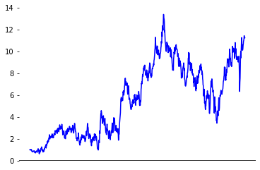
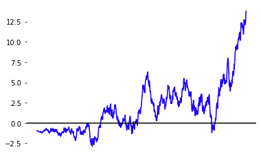
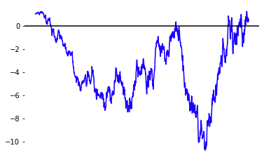
If you are familiar with stochastic calculus, the marginal distribution of \(X_t\) is equivalent to sampling \(X_t\) using the stochastic differential equation \(dX = \sqrt{2t} \, dW_t\). The term diffusion comes from physics, where particles move around under random motion represented by this SDE. If you are not yet familiar with stochastic calculus, fear not! Much of the mathematics of diffusion can be understood without it, and we will introduce stochastic calculus later.
The model consists of a denoiser \(D = D(x, t)\) where \(x, t \in \R\) are scalar values, possibly represented as a neural network \(D = D_\theta\) with parameters \(\theta\). We train it with a mean square error loss, on predicting the ground truth unnoised value \(X_0\) given that the denoiser sees the noised value \(X_t\):
\[\begin{equation} \label{eq:intro_loss_defn_of_denoiser} \text{loss} = \E | D(X_t, t) - X_0 |^2 \end{equation}\](The expectation is over \(t\), \(X_0\), and \(X_t\), for some distribution over times \(t\). We haven’t yet specified what the distribution of \(t\) is, and this is important, but we will defer this as an implementation detail until later.)
Sampling
As \(t \rightarrow \infty\), the distribution of \(X_t\) is approximately Gaussian, and these distributions vary continuously:
Indeed, if we scale by \(1/t\), then it “converges in distribution” to a Gaussian, \(X_t / t \underset{\text{distribution}}{\rightarrow} N(0, 1)\).
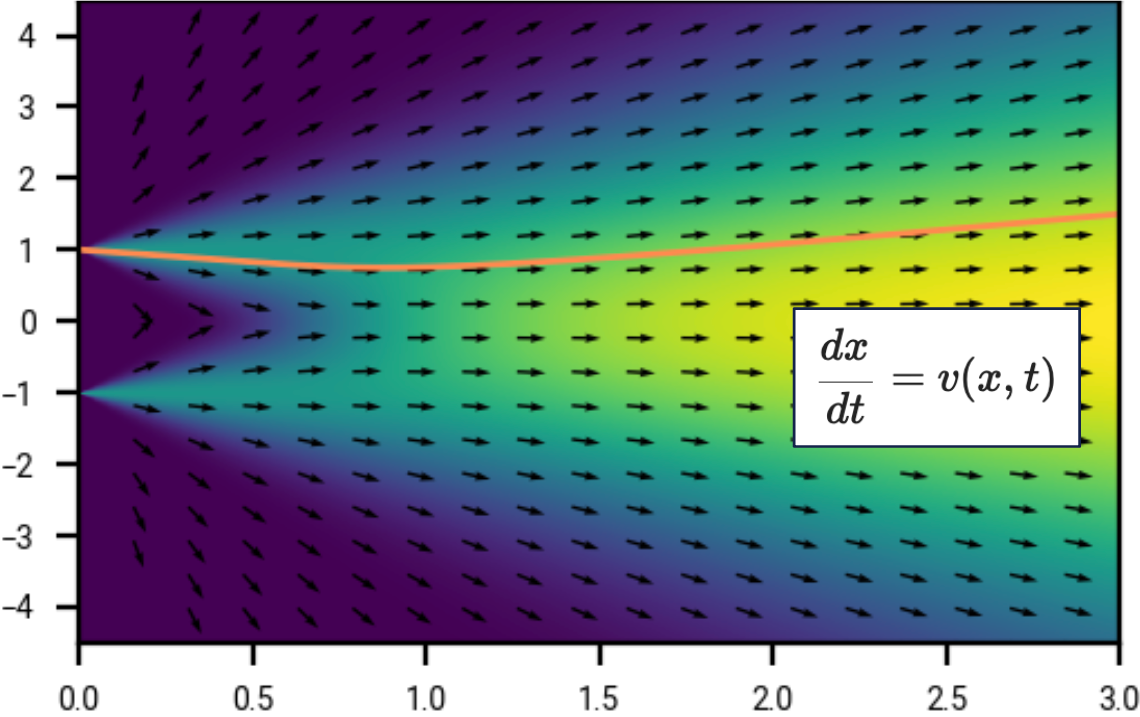
We will later show that since this probability distribution varies continuously as a function of \(t\), that there is a differential equation \(\frac{dx}{dt} = v(x, t)\), such that following trajectories from this differential equation will “preserve the probability”. This means we can (approximately) sample from the original distribution by:
- Start with \(x_T \sim N(0, T^2)\) for \(T\) sufficiently large.
- Integrating \(\frac{dx}{dt} = v(x, t)\) from \(t=T\) to \(t=0\).
This will give us an approximate sample from the original distribution of \(X_0\). What is \(v(x, t)\)? At least for the form of noise that we add, the differential equation turns out to have a particularly simple form:
\[\begin{equation} \label{eq:dx_dt_in_motivating_example} \frac{dx}{dt} = - \frac{D(x, t) - x}{t} \end{equation}\]where \(D\) is the denoiser we trained earlier. We haven’t covered the mathematics of any of this so far; this will come later. But it is magical that this works at all; that we can learn this differential equation using a neural network and a simple loss function.
Recap
During training (forward process), we
- Draw samples from the data distribution.
- Add Gaussian noise \(N(0, t^2)\).
- Train a denoiser \(D(x, t)\) to predict the original using a mean-squared error loss.
During sampling (backward process), we
- Draw samples from the Gaussian \(N(0, T^2)\) for \(T\) sufficiently large.
- Follow the ODE to get a sample from the original distribution.
Exercises
This example was pretty basic, but it introduces a lot of the ideas in generative diffusion models, and we can already build up a lot of intuition by doing some calculations.
In some of the following exercises, the following linear approximations for small \(\vert x \vert\) may be useful:
\[\exp(x) = 1 + x + O(x^2) \qquad \frac{1}{1 + x} = 1 - x + O(x^2)\]Noise destroys information
Given the value for \(X_t = X_0 + N(0, t^2)\), our best guess for the value of \(X_0\) is simply to look at the sign of \(X_t\). How likely is this to be correct?
Using Bayes rule, show that
\[\begin{equation} \label{eq:p_x0_xt} P( X_0 = 1 | X_t > 0) = P(N(0, 1) > -\frac{1}{t}). \end{equation}\]There is no closed form analytic expression for the right hand side, but it can be expressed in terms of the error function \(\text{erf}(z) = \frac{2}{\sqrt \pi} \int_0^z e^{-s^2} ds\).
By writing the above in terms of the error function and using the first order approximation \(\text{erf}(z) = 2z/\sqrt{\pi} + O(z^2)\) or otherwise, deduce that for \(t\) large,
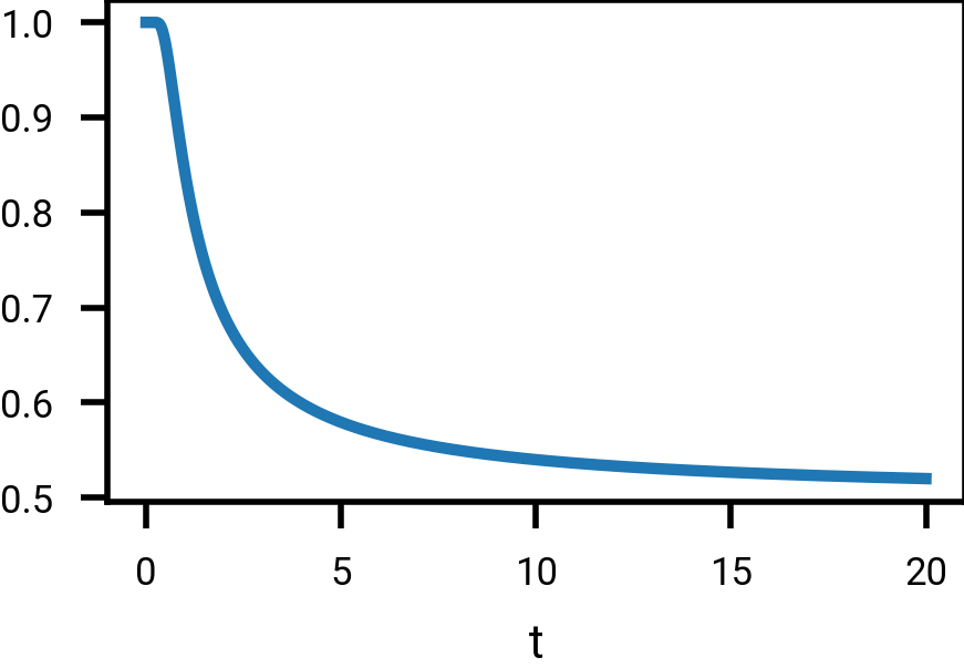
\[P \big( \text{sign}(X_0) = \text{sign}(X_t) \big) \approx \frac{1}{2} + \frac{1}{\sqrt{2\pi} t}.\]Are there any other heuristics we could have used to deduce that this probability is approximately \(1/2 + c/t\) for some \(c>0\) when \(t\) is large?
Thus the probability \(\eqref{eq:p_x0_xt}\) of guessing \(X_0\) correctly based on \(X_t\) tends to \(1/2\), but relatively slowly:
We can be more accurate. If we know \(X_t\), what is the distribution of \(X_0\)?
Show that \(P(X_0 \vert X_t) := P(X_0, X_t) / P(X_t)\) is equal to
\[\begin{equation} \label{eq:p_x0_xt_approx} \frac{1}{1 + \exp(-2 X_0 X_t / t^2)} \approx \frac{1}{2} \left( 1 + \frac{X_0 X_t}{t^2} \right) \end{equation}\]where the second approximation holds provided \(\vert X_t \vert \ll t^2\).
(\(\vert X_t \vert \ll t^2\) holds with high probability as \(t \rightarrow \infty\), i.e., for all \(c>0\), \(P(\vert X_t \vert < c t^2) \rightarrow 1\) as \(t \rightarrow \infty\).)
Using this, we can calculate the mutual information of \(X_0\) and \(X_t\).
Using \(\eqref{eq:p_x0_xt_approx}\), show that the mutual information
\[I(X_0, X_t) = H(X_0) - H(X_0 \vert X_t)\]of \(X_0\) and \(X_t\) when \(t\) is large is
\[\begin{equation} \label{eq:intro:mutual_info} I(X_0, X_t) \approx \frac{1}{t^2 \log 2}. \end{equation}\]Hint: it may be easier to factor the expectation in \(H(X_0 \vert X_t)\) as over \(X_0\) and \(X_t - X_0\).
Thus the mutual information between \(X_0\) and \(X_t\) tends to zero as \(t\) tends to infinity. This is expected: as we add more Gaussian noise, the amount of information about \(X_0\) decreases.
Higher dimensions
The example in this section was for a scalar \(X \in \R\). Typically however diffusion is done in a high-dimensional vector spaces \(X \in \R^n\), where \(n\) may be in the thousands or even millions. What happens if we add noise to the vector \(X_0 1_n\), where \(1_n = (1, \ldots, 1) \in \R^n\) is the all-ones vector?
Let \(X_0\) be a signed Bernoulli random variable as before, and write \(Y_0 = X_0 1_n = (X_0, \ldots, X_0)\). Let
\[Y_t = Y_0 + N(0, t^2 1_n)_{\R^n}\]where \(N(0, t^2 1_n)_{\R^n}\) is the vector of \(n\) independent Gaussians \(N(0, t^2)\). Generalizing Exercise 1.2, show that
\[P(X_0 \vert Y_t) = \frac{1}{2} \prod_{i=1}^n \frac{2}{1 + \exp(-2 X_0 Y_{t,i} / t^2)} \approx \frac{1}{2} \left( 1 + \frac{X_0 \sum_i Y_{t,i}}{t^2} \right)\]where the approximation holds provided \(\sum_i \vert Y_{t,i} \vert \ll t^2\).
Thus for large \(t\), the distribution of \(X_0\) conditioned on \(Y_t\) is approximately determined by \(\sum_i Y_{t,i}\), i.e., this is approximately a sufficient statistic. Since this is distributed as
\[\sum_i Y_{t,i} \sim n X_0 + N(0, nt^2),\]the effect of adding noise independently to \(n\) copies of \(X_0\) is that the effective time gets scaled
\[t \rightarrow t / \sqrt{n}\]when \(t\) is large.
As a curious observation, we can also obtain this result from the exercise on mutual information, specifically, \(\eqref{eq:intro:mutual_info}\). For large \(t\), the \(Y_{t, i}\) are approximately independent, and so \(I(X_0, Y_t) \approx \sum_{i=1}^n I(X_0, Y_{t,i}) \approx n / t^2 \log 2\), again yielding the factor of \(t / \sqrt{n}\).
This is something to be aware of when adding noise to high dimensional inputs:
when there is more redundancy in the unnoised ground truth, more noise needs to
be added to destroy the original signal. For more on this, and further refinements of this idea for images, see [8, 9]Simple diffusion: End-to-end diffusion for high resolution images
Hoogeboom, Emiel and Heek, Jonathan and Salimans, Tim
International Conference on Machine Learning, 2023
On the importance of noise scheduling for diffusion models
Chen, Ting
arXiv preprint arXiv:2301.10972, 2023.

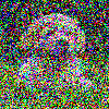
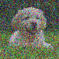
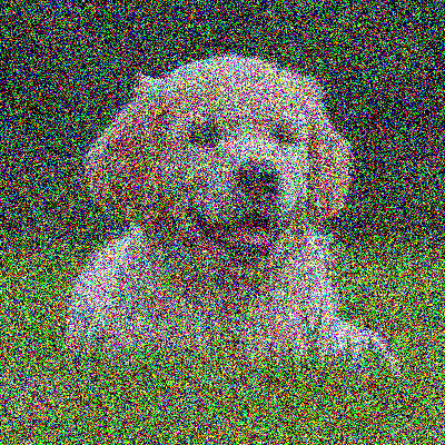
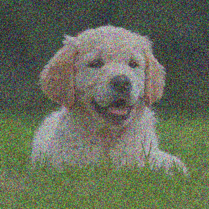
50 × 50
100 × 100
200 × 200
400 × 400
800 × 800
Images with the same amount of per-pixel noise \(N(0, 0.7^2)\) added. Example from Chen et al, 2023. As the image resolution becomes higher, the same amount of per-pixel noise destroys less information about the original image.
Denoiser
The denoiser \(D\) was defined in \(\eqref{eq:intro_loss_defn_of_denoiser}\) as the minimizer of a certain “prediction error”. Assuming this loss is perfectly achieved, i.e., \(D\) is the true mathematical minimizer of \(\eqref{eq:intro_loss_defn_of_denoiser}\), then there is another equivalent definition of the denoiser.
Given \(t>0\), let \(D(\cdot, t) : \R \rightarrow \R\) be the minimizer of the expectation \(\E \vert D(X_t, t) - X_0 \vert^2\).
By expanding the definition of expectation over \(X_0, X_t\) as an integral, show that \(D\) is the conditional expectation
\[D(x, t) = \E [X_0 | X_t = x] := \int P(X_0=x_0 \vert X_t=x) x_0 \, dx_0.\]Hint: we are finding a function that minimizes an integral. This is slightly trickier than standard calculus, and you may find it useful to work from first principles and consider a perturbation \(D'(x_t, t) = D(x_t, t) + \eps \delta(x_t - x_{t'})\) where \(\eps = o(1)\).
Thus the denoiser \(D(x, t)\) gives the expected value of \(X_0\) conditioned on \(X_0 + N(0, t^2) = x\). This is not specific to this example, and is part of a more general phenomenon.
To learn a denoiser \(D_\theta\) parameterized as a neural network, we perform gradient descent on the denoising loss to learn the parameters \(\theta\). Different noise levels \(t\) have different expected error magnitudes. If we naively summed them, then the neural network would dedicate its learning capacity to larger noise levels, and so often the loss includes a term that adjusts for this. What are the typical loss magnitudes at different noise levels?
The precise expected value of the denoiser loss at different noise levels is hard to calculate. But we can estimate reasonable bounds on it.
At low noise levels, \(\hat{D}(x, t) = x\) is a reasonable denoiser. At high noise levels, \(\hat{D}(x, t) = 0\) is a good denoiser. We can interpolate between these two regimes via the denoiser \(\hat{D}(x, t) = \alpha(t) x\). Show that the optimum interpolation value is \(\alpha(t) = 1/(1+t^2)\), and this gives an upper bound on the denoiser loss for an optimum denoiser of
\[\begin{equation} \label{eq:denoiser_upper_bound} \E \vert D(X_t, t) - X_0 \vert^2 \le \frac{t^2}{1+t^2}. \end{equation}\]How tight is this bound?
This estimate for the typical loss magnitude is used to balance the denoising loss contributions at different noise levels. The bound \eqref{eq:denoiser_upper_bound} is used in [10]Elucidating the design space of diffusion-based generative models
Karras, Tero and Aittala, Miika and Aila, Timo and Laine, Samuli
Advances in Neural Information Processing Systems, 2022, and the cruder bound of \(1/t^2\) is used elsewhere e.g. [11, 5, 12]Denoising diffusion implicit models
Song, Jiaming and Meng, Chenlin and Ermon, Stefano
arXiv preprint arXiv:2010.02502, 2020
Score-based generative modeling through stochastic differential equations
Song, Yang and Sohl-Dickstein, Jascha and Kingma, Diederik P and Kumar, Abhishek and Ermon, Stefano and Poole, Ben
arXiv preprint arXiv:2011.13456, 2020
Improved denoising diffusion probabilistic models
Nichol, Alexander Quinn and Dhariwal, Prafulla
International conference on machine learning, 2021.
Continuity
For \(t \ge 0\) we defined \(X_t = X_0 + N(0, t^2)\). We didn’t specify the joint independent structure of the different \(X_t\), but we can look at the marginal probability density function \(\rho(x, t)\) for every \(t \ge 0\). Observe that \(\rho(x, t)\) is a point mass at \(x=0\) when \(t=0\), but is otherwise spread out over all of \(\R\) for \(t > 0\). Thus \(\rho\) has a singularity and is “discontinuous” at time \(t=0\). Actually, it’s not even a standard function here (since it takes “infinite value”), although it does exist in the space of generalized functions, where
\[\rho(x, 0) = (\delta(x-1) + \delta(x+1))/2\]and \(\delta(x)\) is the delta mass function that obeys \(\int \delta(x) f(x) dx = f(0)\).
Despite the probability density function being discontinuous at \(t=0\), there’s a sense in which the sequence of distributions is still continuous for all \(t\).
Let \(F : \R \rightarrow \R\) be a continuous function with compact support (this means that \(F(x) = 0\) for sufficiently large \(\vert x \vert\)). Show that
\[t \mapsto \E F(X_t) = \int \rho(x, t) F(x) dx\]is continuous in \(t\) for all \(t \ge 0\).
In the above, the function \(F\) is known as a test function: we can “test” the distribution to see how it acts. (Sometimes test functions also have additional constraints, such as having continuous derivatives.)
Let \(Z \equiv N(0, 1)\) be a Gaussian random variable. Show that for any test function \(F : \R \rightarrow \R\), that
\[\E F(X_t / t) \rightarrow \E F(Z)\]as \(t \rightarrow \infty\). We say that \(X_t / t\) converges in distribution to \(N(0, 1)\).
Final remarks
The signed Bernoulli distribution is a very simple distribution: it is one dimensional, and is entirely symmetric about zero, consisting of two discrete points. During the sampling process, if we follow the ODE \(\eqref{eq:dx_dt_in_motivating_example}\) backwards starting from an initial point \(X_T\), then where we end up depends only on the sign \(\text{sign}(X_T)\). The space \(\R\) is thus partitioned into \(\{x > 0\}\) and \(\{x < 0\}\), with \(\{x > 0\}\) mapped to \(x=+1\) and \(\{x < 0 \}\) mapped to \(x=-1\). (The point \(X_T=0\) gets mapped to \(x_0=0\) under this ODE, but the set \(\{0\}\) has measure zero so is ignorable when considering transformations of distributions.)
What is more magical about diffusion is that following this ODE allows transformations of simple Gaussians to far more complex distributions in a continuous and probability-preserving manner.
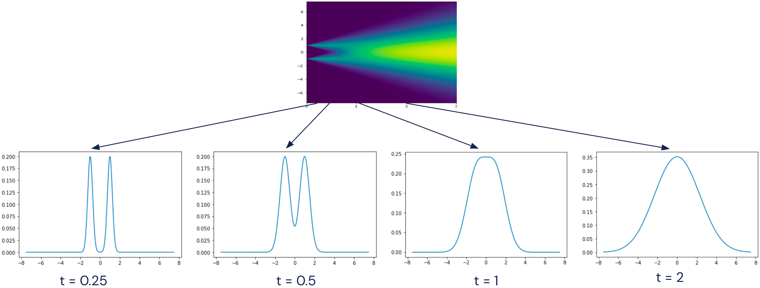
What does this look like for a slightly more complex \(X_0\), consisting of three points at \(\{(-1, +1), (+1, -1), (+1, +1)\}\)? This is harder to picture, but below shows the probability density as a function of time, with time running backwards, starting from a distribution at time \(t=3\) which is approximately Gaussian, and converging to this discrete distribution.
Visualizing the probability density of three points with Gaussian noise added, together with the vector field of the differential equation \(\eqref{eq:dx_dt_in_motivating_example}\). The right hand image is a zoomed in version of the left. Initially the vector field (given by the denoiser) points to the mean of the three points. At some point, there is ‘symmetry breaking’, and the arrows starts to converge around their nearest point.
(There is some numerical instability in drawing the vector field: close to time \(t=0\), the magnitude of the ODE flow away from the initial points is very large.)
We can start to see how diffusion might work for more complex data distributions, such as natural images, which live in very high dimensional spaces. During sampling we start at sufficiently large \(T\) where the sample looks like noise, and then gradually resolve details as we go backwards through time.
In the next section we introduce some formalism around stochastic processes, which is useful for talking about families of random variables.