5. Numerical integration
Recall the results of the previous section: we have shown that if we sample \(X_0\) from the data distribution, and let \(X_t = X_0 + N(0, t^2 I)\), then the probability flow ODE \(\frac{dx}{dt} = v(x, t)\) where \(v(x, t)\) is given by Exercise 4.3 preserves the marginal density \(\rho(x, t)\) of the \(X_t\).
Thus we now have a means of sampling from the data distribution at \(t=0\) provided we have a denoiser that yields \(v\).
Suppose we have a time-indexed family of distributions given by the probability density function \(\rho(x, t)\), and that \(v\) is a drift for \(\rho\) (i.e., \(v\) and \(\rho\) satisfy the continuity equation). Suppose further we can approximately sample from \(\rho(x, t_0)\) for \(t_0\) large.
The strategy for generating a sample from \(\rho(x, 0)\) is as follows.
- Sample from the approximate distribution for \(\rho(x, t_0)\), for example, \(x(t_0) \sim N(0, t_0^2)\).
- Starting from \((x(t_0), t_0)\), numerically integrate \(v(x, t)\) to obtain an approximation to the trajectory \(\Phi(t; x(t_0), t_0)\) which would yield a sample \(\Phi(0; x(t_0), t_0)\) from \(\rho(x, 0)\).
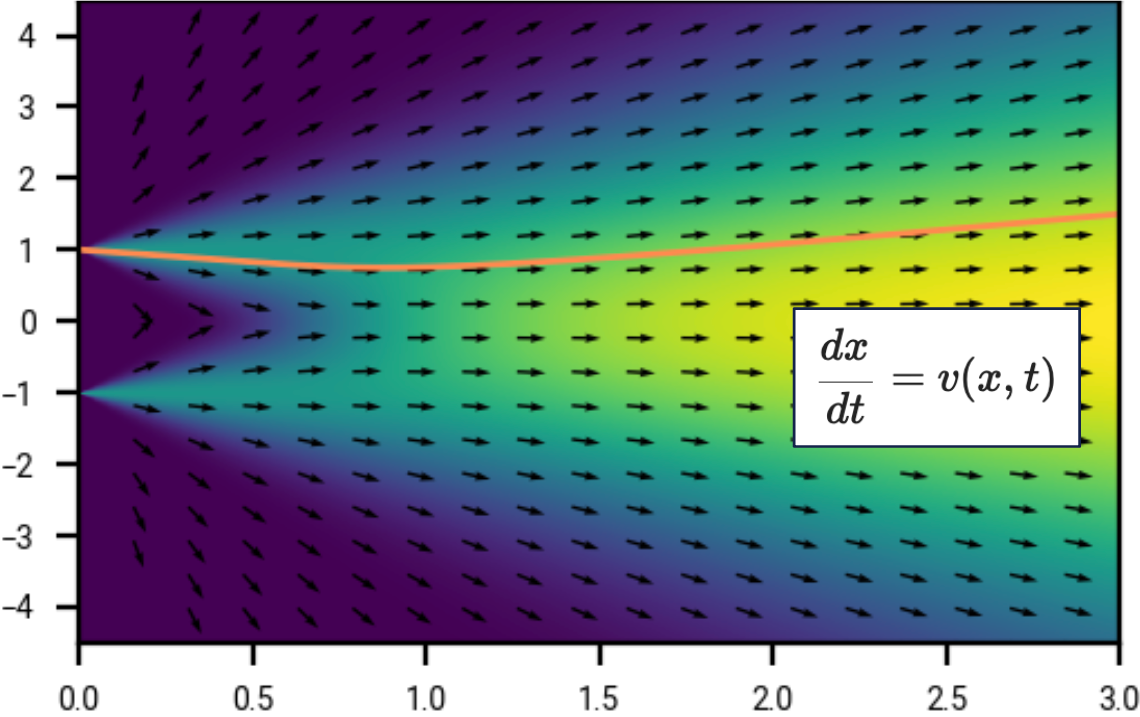
This shows a trajectory (orange) in the sample space \(\R\), and in this example our final sample is 1. Note the velocity or drift field \(v\), shown by the black arrows, points to the right; we take negative time steps to arrive at a sample at \(t=0\).
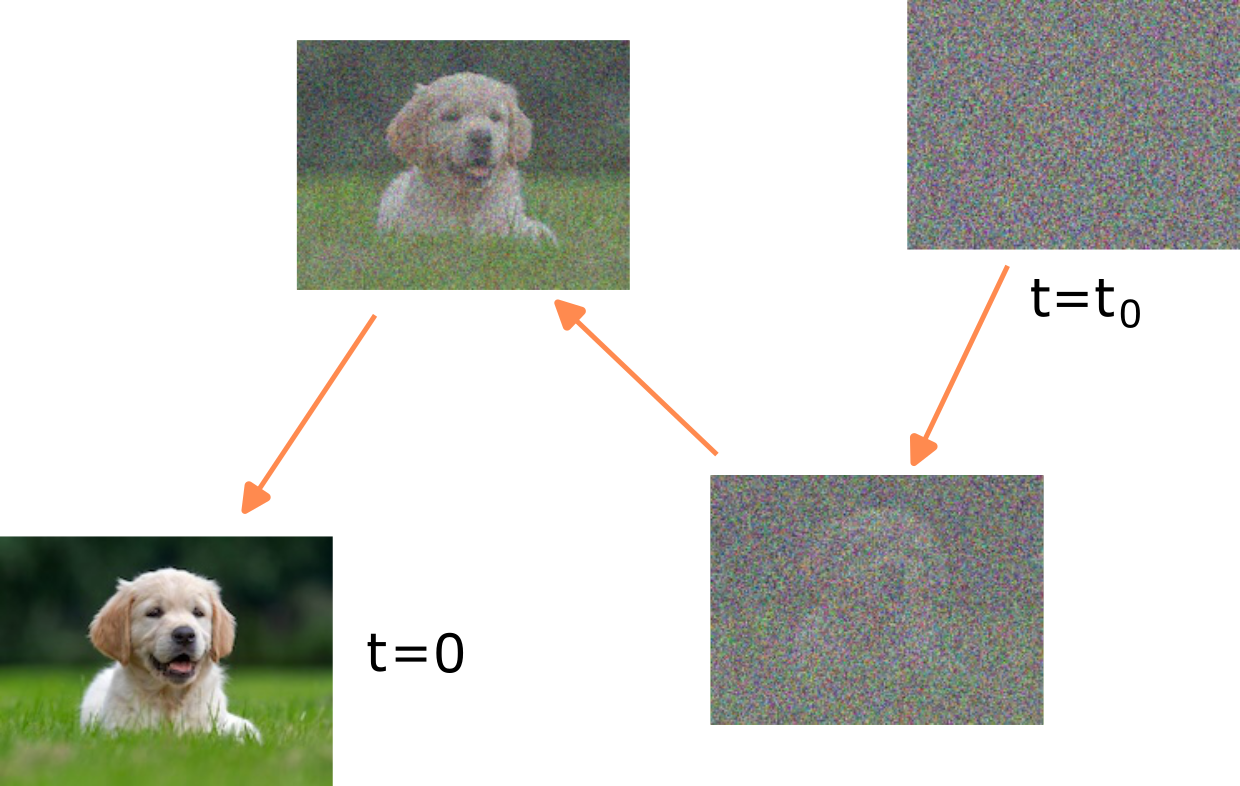
An example of what integration looks like for a real-life example, in the (much) higher dimensional vector representing the space of images. A sample at large \(t_0\) looks like random Gaussian noise. As we integrate backwards-in-time, following the velocity \(v\) given by the denoiser \(D\), the image gradually emerges.
Integration involves sampling a point for \(t_0\) sufficiently large from the distribution with density function \(\rho(\cdot, t_0)\) and following the probability flow ODE backwards.
Thus conceptually, deterministic sampling is straightforward. However, in practice we must numerically integrate \(v\). In this section we consider this, in particular numerical integration errors.
Numerical integration algorithms
The simplest way of integrating \(v(x, t)\) is using Euler’s first order method. Given \(n \ge 1\) and time steps \(t_0 > t_1 > \cdots > t_n = 0\), Euler integration is
\[\begin{equation} \label{eq:euler_integration} x_{i+1} = x_i + (t_{i+1} - t_i) v(t_i, x_i). \end{equation}\]The final sample is \(x_n\). (Sometimes instead for the final sample, we take the denoiser predictions from the denoiser \(D\).)
Note that time is decreasing as a function of the time index; this can be confusing, but is consistent with how we have used \(t_0\) to define trajectories, as well as the EDM convention [10]Elucidating the design space of diffusion-based generative models
Karras, Tero and Aittala, Miika and Aila, Timo and Laine, Samuli
Advances in Neural Information Processing Systems, 2022.
There are various sources of error in this:
- The distribution of \(x_0\) might not be precisely the same as \(\rho(\cdot, t_0)\) (e.g., if there is a mismatch from it being a true Gaussian).
- Numerically integrating \(v(x, t)\) yields an integration error.
- The function \(v(x, t)\) might not be precisely a drift consistent with \(\rho\) (e.g., if it arises from an imperfect denoiser).
Analyzing the integration error
For this part, let’s fix \(t_0\) and \(x_0\). Let \(\phi(t)\) be the true trajectory that arises from (non-numerically) integrating \(v(x, t)\) from \(t_0\) down to \(t_n\). Thus \(\phi(t_0) = x_0\) and \(\phi'(t) = v(\phi(t), t)\) for \(t_n \le t \le t_0\).
Errors in Euler integration accumulate over many timesteps. Each integration step induces a local error, where even if we were to start at the correct position \(x_i = \phi(t_i)\), we accumulate a small error. Global error then results from the accumulation of these local errors and the effect of evaluating \(v\) at a point \(x_i \ne \phi(t_i)\).
The single-step error is
\[\begin{equation} \phi(t_{i+1}) - \phi(t_i) - (t_{i+1} - t_i) v(t_i, \phi(t_i)) \end{equation}\]and is called the local truncation error.
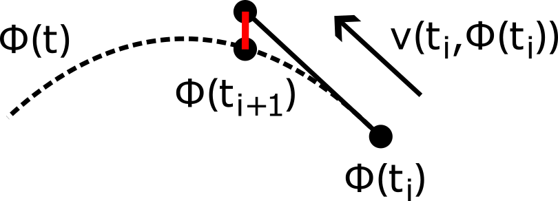
Local truncation error, shown in red.
The word “truncation” signifies that this error is due solely to Euler’s method, and does not include any effects due to e.g., floating point approximations. The local truncation error can be estimated using the Taylor expansion of \(\phi\). Indeed, writing \(h_i = t_{i+1} - t_i\) and using \(\phi'(t_i) = v(t_i, \phi(t_i))\), the local truncation error is
\[\begin{align} \nonumber \phi(t_{i+1}) - \phi(t_i) - h_i v(t_i, \phi(t_i)) &= (\phi(t_i) + h_i \phi'(t_i) + \frac{1}{2} h_i^2 \phi''(t_i) + O(h_i^3)) - \phi(t_i) - h_i \phi'(t_i) \\ \label{eq:local_truncation_error_bound} &= \frac{1}{2} h_i^2 \phi''(t_i) + O(h_i^3) \end{align}\]In particular, the local truncation error is quadratic in the timestep. How do these local errors accumulate?
The (signed) error in \(x_i\) is \(\phi(t_i) - x_i\) and is called the global truncation error at time \(t_i\).
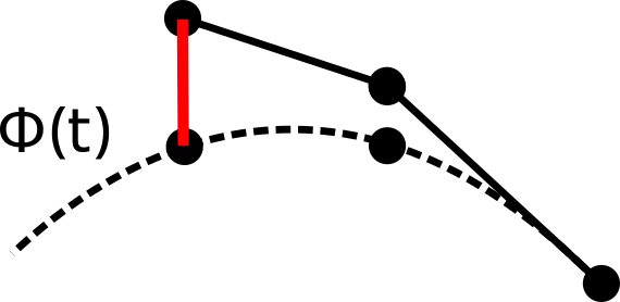
Global truncation error over several steps, shown in red.
Write this error as \(\epsilon_i = \phi(t_i) - x_i\). It is possible to inductively bound \(\epsilon_{i+1}\) in terms of \(\epsilon_i\); we sketch the details. Observe that
\[\begin{align*} \epsilon_{i+1} &= \phi(t_{i+1}) - x_{i+1} \\ &= \phi(t_{i+1}) - x_i - h_i v(t_i, x_i) \\ &= [{\color{red} \phi(t_i)} - x_i] + [\phi(t_{i+1}) - {\color{red} \phi(t_i)} - h_i {\color{blue} v(t_i, \phi(t_i))}] + h_i [{\color{blue} v(t_i, \phi(t_i))} - v(t_i, x_i)] \end{align*}\]The first \([\cdots]\) is just \(\epsilon_i\). The second \([\cdots]\) is just the local truncation error, which is bounded by \eqref{eq:local_truncation_error_bound}. Finally, the third \([\cdots]\) is by Taylor expansion bounded by \(\vert \epsilon_i \vert \,\textrm{sup}_x \vert\vert\nabla v(x, t_i)\vert\vert\) .
It is then possible to do a standard inductive summation argument to yield \(\vert\epsilon_i\vert \le \frac{A}{2B} [ \exp\{B(t_i-t_0)\} - 1] \max_i \epsilon_i\) where \(A\) and \(B\) are constants that depend on \(v(x, t)\).
Having good bounds on the global integration error is a hard problem, and finding the optimal sequence of \(t_i\) that minimizes the integration error is an empirical question. However, observe that the bound \eqref{eq:local_truncation_error_bound} for the local integration error suggests we should have tighter spacing of timesteps when \(\phi''(t)\) is larger. This is likely to be at intermediate noise levels; c.f. Exercise 3.2.
Higher-order integrators
We can also use higher-order integrators, which offer better errors as a function of the number of NFA evaluations. [10]Elucidating the design space of diffusion-based generative models
Karras, Tero and Aittala, Miika and Aila, Timo and Laine, Samuli
Advances in Neural Information Processing Systems, 2022 propose using an explicit 2nd-order Runge-Kutta method. This replaces \eqref{eq:euler_integration} with the following update, where \(h_i = t_{i+1} - t_i\), and \(\alpha > 0\) is a parameter, where \(\alpha = 1\) corresponds to Heun’s method, and \(\alpha=1/2\) and \(\alpha=2/3\) correspond to midpoint and Ralston methods respectively.
Here we use Taylor approximations to analyze the local truncation error.
-
For simplicity, suppose at first that \(v\) has no dependence on \(x\), i.e., \(v=v(t)\). In this case, \(\phi''(t) = v'(t)\). By using the Taylor expansions of \(\phi\) and \(v\) as
\[\begin{align*} \phi(t+h) &= \phi(t) + h \phi'(t) + \frac{1}{2} \phi''(t) + O(h^3) \\ v(t+h) &= v(t) + h v'(t) + O(h^2) \\ &= \phi'(t) + h \phi''(t) + O(h^2) \end{align*}\]and substituting these into \eqref{eq:2nd_order_integration}, show that the local truncation error \(\phi(t_{i+1}) - x_{i+1}\) when \(x_i = \phi(t_i)\) is \(O(h_i^3)\) for all choices of \(\alpha = O(1)\). (Thus the local truncation error is cubic, rather than quadratic in \(h_i\), compared with the Euler method.)
-
In the general case where \(v=v(x, t)\) has a dependence on \(x\), use the result of Exercise 3.2 for \(\phi''(t)\) and the Taylor expansion of \(v\) to show that the local truncation error is again \(O(h_i^3)\) for \(\alpha=O(1)\).
Spacing of timesteps? A worked example
Let’s suppose we have a fixed compute budget (corresponding to the number of integration steps \(n\)), and want to minimise the integration error. How should we space the timesteps \(t_i\)?
Let’s look at a worked toy example. This example is basic, but it has some features in common with world setups. We will start with a highly simplified setup where we work entirely in the space \(\{-1, 1\}^n\) with boolean noise, and then extend to adding Gaussian noise in the larger ambient \(\R^n\).
Let the data distribution of \(X_0\) be the uniform distribution \(X_0 \sim U_\mathcal{A}\) over a random subset \(\mathcal{A}\) of the boolean hypercube \(\{-1, 1\}^n\). (We use \(\{-1, 1\}\) rather than \(\{0, 1\}\) because this is more in keeping with conventions elsewhere, including the example in the introduction.)
More precisely, let \(0 <p < 1\), and let \(\mathcal{A} \subset \{-1, 1\}^n\) be a random subset where each point is included with probability \(p\). Let \(X_0\) have uniform distribution
\[p_{X_0}(x) = \begin{cases} 1 / |\mathcal{A}| \quad & \text{if } x \in \mathcal{A}, \\ 0 & \text{otherwise}. \end{cases}\]In this, we make repeated use (sometimes implicitly) of the idea of concentration of measure.
We generated \(\mathcal{A} \subset \{-1, 1\}^n\) by including each element with probability \(p\). The expected size of \(\mathcal{A}\) is \(\E \vert \mathcal{A} \vert = p2^n\). This can be written as \(\vert \mathcal{A} \vert = \sum_{x \in \{-1, 1\}^n} 1_{x \in \mathcal{A}}\). Each \(1_{x \in \mathcal{A}}\) is a random variable, with value between \(0\) and \(1\), and with expected value \(p\). Concentration of measure is the remarkable phenomena that assuming the random variables \(1_{x \in \mathcal{A}}\) are sufficiently independent (and in this case they are fully independent), that the sum \(\vert \mathcal{A} \vert\) concentrates in a much narrow range than \(O(2^n)\), typically in a range proportional to the square root of the number of random variables. This can be made quantitative through a variety of large deviation inequalities.
In our case, \(\vert \mathcal{A} \vert = p2^n + o(n)\) with very high probability (i.e., with probability tending to 1) as \(n \rightarrow \infty\).
For a much broader and informal introduction to concentration of measure, see Sander’s post on typicality [16]Musings on typicality
Dieleman, Sander
https://benanne.github.io/2020/09/01/typicality.html.
Let’s add noise to \(X_0\). For now we will use the simplified setup of adding Bernoulli noise to each component of \(X_0\); this keeps us in the space \(\{-1, 1\}^n\) (rather than adding Gaussian noise in \(\R^n\)). More precisely, given \(0 \le q \le 1\), let \(X_q \in \{-1, 1\}^n\) be \(X_0\) where each component has been corrupted with an i.i.d. Bernoulli variable \(\text{Be}(q)\):
\[X_{q, i} = \begin{cases} X_{0, i} \quad & \text{with probability } 1 - q,\\ - X_{0, i} \quad & \text{otherwise.} \end{cases}\](Thus for example \(X_1 = - X_0\).) We can write this more compactly as \(X_q = X_0 \odot \text{Be}(q)_n\).
What’s the mutual information between \(X_0\) and \(X_q\), as a function of \(q\)? We can estimate it, using an argument similar to the proof of Shannon’s theorem on noisy channels. The argument isn’t fully rigorous, but it can be made precise.
For \(x, y \in \{-1, 1\}^n\), let \(d(x, y) = \sum_i 1_{x_i \ne y_i}\) be the Hamming distance between \(x\) and \(y\), counting the number of differing coordinates.
-
Show that
\[\E d(X_0, X_q) = qn.\]Thus by concentration of measure, \(d(X_0, X_q) = (q + o(1))n\) with high probability.
-
Show that the number of points in \(\{-1, 1\}^n\) that are at distance \((q + o(1))n\) from \(X_q\) is (with high probability)
\[2^{(H_2(q) + o(1))n}\]where \(H_2(q) = -q \log_2 q - (1-q) \log_2 (1-q)\) is the binary entropy function, and where \(o(1) \rightarrow 0\) as \(n \rightarrow \infty\).
-
Thus conditioned on \(X_q\), with high probability \(X_0\) is at distance \((q + o(1))n\) from \(X_q\). By estimating the number of points in \(\mathcal{A}\) “close” to \(X_q\), deduce that the entropy of \(X_0\) conditioned on \(X_q\) is
\[\begin{equation} \label{eq:entropy_X0_cond_on_Xq} H(X_0 | X_q) = \max \big\{ 0, \log_2 |\mathcal{A}| - (1 - H_2(q)) n \big\} + o(n) \end{equation}\]and in particular the mutual information is
\[\begin{equation} \label{eq:mutual_info_X0_Xq} I(X_0, X_q) = \min \big\{ \log_2 |\mathcal{A}|, (1 - H_2(q)) n \big\} + o(n). \end{equation}\]
What does the entropy \eqref{eq:entropy_X0_cond_on_Xq} of \(X_0\) conditioned on \(X_q\) look like as a function of \(q\)? In the range \([0, q^*]\) where \(0 < q^* < 1/2\) is the solution to
\[H_2(q^*) = 1 - \log_2 \vert \mathcal{A} \vert / n,\]the entropy is \(o(1)\) with high probability. I.e., up to noise level \(q^*\), adding Bernoulli noise does not destroy any information at all about \(X_0\).
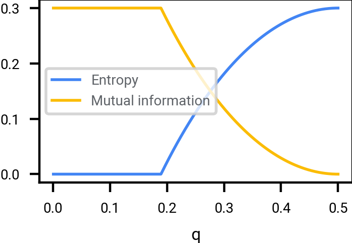
Mutual information, and entropy, scaled by \(1/n\), between \(X_0\) and \(X_q\) where \(X_0\) is a uniformly selected point of \(\mathcal{A} \subset \{-1, 1\}^n\), and where (for the plot above) \(\vert \mathcal{A} \vert \approx 2^{0.3 n}\), in the limit \(n \rightarrow \infty\). Adding Bernoulli noise up to \(q^* \approx 0.1893\) destroys zero information about \(X_0\) in this limit.
Note also that if we extend past \(q=1/2\), then plot is mirrored. This is an artifact of using Bernoulli noise. For example, \(q=1\) corresponds to perfectly flipping the bits, which destroys zero information. (If we added Gaussian noise, then we would not get this mirroring behavior.)
In the example so far, we added Bernoulli noise: \(X_q = X_0 \odot \text{Be}(q)_n\). What happens if instead we add Gaussian noise
\[\begin{equation} \label{eq:add_gaussian_to_binary_vector} X_t = X_0 + N(0, t^2)_{\R^n} \end{equation}\]It is in fact possible to “convert” the Gaussian noise to an equivalent amount of Bernoulli noise, i.e., find \(q=q(t)\) such that adding \(\text{Be}(q)\) destroys an equivalent amount of information to adding \(N(0, t^2)\). The formula for \(q(t)\) is not analytic, but can be computed numerically, and estimated asymptotically.
For this exercise, let \(n=1\), so that \(X_0\) is uniformly sampled from \(\{-1, 1\}\). Let \(Y_q = X_0 \oplus \text{Be}(q)\) and let \(Z_t = X_0 + N(0, t^2)\). Can we solve for \(I(X_0, Y_q) = I(X_0, Z_t)\) when \(t\) is large?
From the argument that gave \eqref{eq:mutual_info_X0_Xq}
\[I(X_0, Y_q) = 1 - H_q(2)\]and from Exercise 1.3:
\[\begin{equation} \label{eq:intro:mutual_info} I(X_0, Z_t) \approx \frac{1}{t^2 \log 2}. \end{equation}\]By using the approximation \(\log (1 + \eps) = \eps + O(\eps^2)\), and the substitution \(q = (1 - \eps)/2\), deduce that
\[q(t) \approx \frac{1 - 1/t}{2}\]when \(t\) is large.
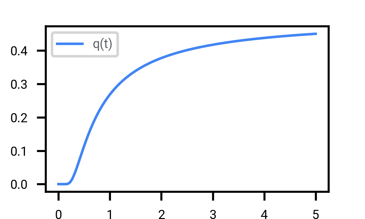
How much Bernoulli noise \(\text{Be}(q)\) is equivalent to a given amount of Gaussian noise \(N(0, t^2)\). As \(t \rightarrow \infty\), \(q(t) \rightarrow (1 - 1/t) / 2\), tending towards to perfect destruction of information.
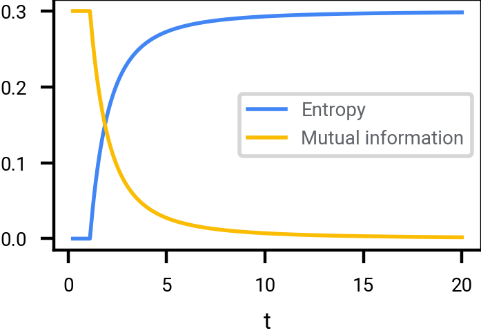
The following figure shows how information about the original sample \(X_0 \equiv U(\mathcal{A})\) is destroyed, for different sized sets \(\mathcal{A} \subset \{-1, 1\}^n\).
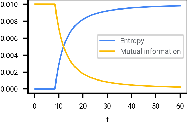
\(\vert \mathcal{A} \vert \approx 2^{0.01 n}\). Observe that much larger values of \(t\) are required to destroy the same amount of information about \(\mathcal{A}\); since \(\mathcal{A}\) is smaller, it is more robust or decodable.
Mutual information, and entropy, scaled by \(1/n\), between \(X_0\) and \(X_t\) where \(X_0\) is a uniformly selected point of \(\mathcal{A} \subset \{-1, 1\}^n\), in the limit \(n \rightarrow \infty\). For finite values of \(n\), the actual curves would be slightly more rounded.
Two things that stand out in adding Gaussian noise to a point sampled from a random set of discrete points:
- At low noise levels, no information is destroyed at all. The original signal is perfectly recoverable.
- The amount of noise \(t\) required to destroy most of the information depends on how sparse the discrete set is. There is no one-size-fits-all solution.
How does this relate to spacing of timesteps?
There are various heuristics to determine the spacing of timesteps in numerical integration, including:
- The timesteps should correspond to “decoding a constant rate of information” (since this is a rate-limiting step by a finite capacity neural network), for example as done in [17]Continuous diffusion for categorical data
Dieleman, Sander and Sartran, Laurent and Roshannai, Arman and Savinov, Nikolay and Ganin, Yaroslav and Richemond, Pierre H and Doucet, Arnaud and Strudel, Robin and Dyer, Chris and Durkan, Conor and others
arXiv preprint arXiv:2211.15089, 2022. - The timesteps should be more heavily concentrated in regions of greater trajectory curvature (since this leads to numerical integration error).
Let \(\mathcal{A} \subset \{-1, 1\}^n\) be a random subset with size \(\vert \mathcal{A} \vert = 2^{\alpha n}\) where \(0 < \alpha < 1\), and let \(X_0\) be a randomly chosen point of \(\mathcal{A}\) (as before), and \(X_t \equiv X_0 + N(0, t^2)\).
Following \eqref{eq:intro:mutual_info} and \eqref{eq:mutual_info_X0_Xq}, assume the mutual information is approximately
\[I(X_0, X_t) \approx \min \big\{ \log_2 \vert \mathcal{A} \vert, \frac{n}{t^2 \log 2} \big\}.\]Given \(N \ge 1\), how should the timesteps \(t_0, t_1, \ldots, t_N\) be spaced so that the “information increments” are uniformly spaced?
In practice, the actual best noise schedule to use is an empirical question, as it is affected by so many things.
For the purpose of denoising images (which can be quite a different setup to denoising a random subset of the boolean hypercube, although certain intuitions carry over), [10]Elucidating the design space of diffusion-based generative models
Karras, Tero and Aittala, Miika and Aila, Timo and Laine, Samuli
Advances in Neural Information Processing Systems, 2022 propose using
for constants \(0 < T_\min < T_\max\) and \(p > 1\).
For a much wider discussion of these issue, see [18]Noise schedules considered harmful
Dieleman, Sander
https://sander.ai/2024/06/14/noise-schedules.html.
Numerical issues
It is common practice in machine learning to use reduced floating point precision (for example 16 rather than 32 bits) to reduce the costs of computation, for example, in computing the activations in a forward pass through a neural network. However, it is recommended to use a high precision floating point format (such as float32) for storing and manipulating the actual intermediate integration values \(x_i\).
The bfloat16 floating-point format is a float point format with 16 bits of precision, and in particular with 7 bits of mantissa. This means that for every range \([2^k, 2^{k+1})\) there are \(2^7 = 128\) values that bfloat16 can take, e.g., close to \(1\) it has approximately two decimal points of accuracy.
What are the values of successive timesteps \(t_i / t_{i+1}\) for either Exercise 5.4 or \eqref{eq:edm_timesteps}?
How might using reduced floating point precision affect numeric integration?