4. Deterministic diffusion for Gaussian noise
In diffusion and generative modelling we want to transform one distribution to another. We can achieve this by continuously interpolating between the two distributions, for example by adding varying amounts of Gaussian noise to the data distribution (such as the space of natural images), and having a method for transforming samples from these corresponding distributions.
The time-indexed family of distributions corresponding to the interpolation has a corresponding time-parameterized density function \(\rho(x, t)\), where \(\rho(x, 0)\) is the probability density of the data distribution, and \(\rho(x, t_0)\) is the probability density of the sampling distribution, such as a multivariate Gaussian. By convention, we place the data distribution at \(t=0\), and integrate “backwards in time” from the sampling distribution for some \(t_0 > 0\).
For the purpose of generative modelling, one way of transforming samples is by integrating the probability flow ODE
\[\begin{equation} \label{eq:stochastic_ode} \frac{dX_t}{dt} = v(X_t, t). \end{equation}\]The question then becomes: given the definition of a sequence of distributions (e.g., arising from adding Gaussian noise), with corresponding densities \(\rho(x, t)\), can we find \(v(x, t)\) such that integrating this probability flow ODE yields this target density \(\rho(x, t)\)? (Hint: this is where the denoiser that we saw in the introduction will come in.)
Time-indexed families of distributions
Recall the continuity equation from the previous section:
\[\begin{equation} \label{eq:continuity_equation} \partial_t \rho(x, t) = - \nabla \cdot \big( \rho(x, t) \, v(x, t) \big) \end{equation}\]The next corollary says that to find \(v\) such that integrating \(v\) gives some desired \(\rho\), it is sufficient to prove that \(v\) and \(\rho\) satisfy the continuity equation. We state and prove this corollary, and then in this section we look at finding \(v\) for various interpolating distributions (such as adding Gaussian noise).
Let \(v : \R^n \times \R \rightarrow \R^n\) and \(\rho : \R^n \times \R \rightarrow \R\) be functions that satisfy the continuity equation \eqref{eq:continuity_equation}. Let \((X_t)_{t \in I}\) for a time interval \(I \subset \R\) be the stochastic process that satisfies
\[\frac{dX_t}{dt} = v(X_t, t)\]with the probability density of \(X_{t_0}\) equal to \(\rho(\cdot, t_0)\) for \(t_0 \in I\).
Then the probability density of \(X_t\) is \(\rho(\cdot, t)\) for \(t \in I\).
Let \(\tau(\cdot, t)\) be the probability density of \(X_t\). By construction \(\tau(\cdot, t_0) = \rho(\cdot, t_0)\), and by Theorem 3.3 \(v\) and \(\tau\) satisfy the continuity equation. Our aim is to prove that \(\rho = \tau\), i.e., that there is a unique solution \(\rho\) to the continuity equation involving \(v\).
Write \(\pi = \rho - \tau\). Since \(\partial_t \rho = -\nabla \cdot (\rho v)\) and \(\partial_t \tau = -\nabla \cdot (\tau v)\),
\[\partial_t \pi(x, t) = 0.\]Since \(\pi(x, t_0) = \rho(x, t_0) - \tau(x, t_0) = 0\), we have that \(\pi\) is in fact zero for all \(t\), and thus \(\rho = \tau\) as required.
Thus given functions \(\rho\) and \(v\), call \(v\) a drift or velocity for \(\rho\) if it obeys the continuity equation \eqref{eq:continuity_equation}.
Observe that via the substitution \(w(x, t) = \rho(x, t) v(x, t)\), finding \(v\) that satisfies the continuity equation is equivalent to solving
\[\nabla \cdot w(x, t) = - \partial_t \rho(x, t).\]Verify that for \(n \ge 2\) dimensions, there exist non-zero \(w\) such that \(\nabla \cdot w = 0\), and thus multiple solutions to the continuity equation. What do these physically correspond to?
What happens in \(n=1\) dimension?
Given a sequence of distributions with probability density \(\rho(x, t)\) where \(t\) ranges over some interval \(I \subset \R\), there are thus many stochastic processes \((X_t)_{t \in I}\) with marginal density given by \(\rho\), since there are many distinct \(v\) which solve \(\eqref{eq:continuity_equation}\).
There are even more \(v\) if we only care about the initial and final distributions at time \(t=0\) and \(t=t_0\).
Often one will want to find \(v\) such that the resulting map has some optimal property, for example, having low curvature which allows for low-step numerical integration (this is the idea behind consistency diffusion). Transportation theory looks at the more general problem of finding mappings between distributions that optimize some objective, and this is a deep mathematical field that we do not cover here.
Convolved distributions
Consider the canonical diffusion example: adding Gaussian noise to an initial distribution. Let \(\pi : \R^n \rightarrow \R\) be the density function of the data distribution, corresponding to \(t=0\). Let
\[\begin{equation} \label{eq:gaussian_noise_t} \tau(x, t) = \frac{1}{(2 \pi)^{n/2} t} \exp \left\{ - \vert \vert x \vert \vert^2 / 2 t^2 \right\} \end{equation}\]be the density of a multivariate Gaussian with variance \(t^2 1_n\). Then the convolution
\[\begin{equation} \label{eq:spatial_convolution_with_time} \rho(x, t) = (\pi * \tau(\cdot, t))(x) := \int_{\R^n} \pi(y) \tau(x - y, t) dy \end{equation}\]corresponds to the time-indexed family of distributions given by adding Gaussian noise with variance \(t^2\) to the initial distribution given by \(\pi\). (The convolution formula above of course holds for general \(\tau\), not just Gaussian noise.)
Verify that \(w(x, t) = x / t\) satisfies the continuity equation for \(\tau\) defined in \eqref{eq:gaussian_noise_t}.
The main result is that if we have \(w\) that satisfies the continuity equation for \(\tau\), we can derive \(v\) that satisfies the continuity equation for the convolved distribution \(\rho\).
Let \(w : \R^n \times \R \rightarrow \R^n\) and \(\tau : \R^n \times \R \rightarrow \R\) satisfy the continuity equation
\[\partial_t \tau(x, t) = - \nabla \cdot (\tau(x, t) w(x, t)).\]Let \(\pi : \R^n \rightarrow \R\) be an “initial distribution”. Let \(v : \R^n \times \R \rightarrow \R^n\) be the minimizer of
\[\begin{equation} \label{eq:convolved_drift_loss} \underset{\substack{ z \sim \pi(z) \\ y \sim \tau(y, t) }}{\E} \vert\vert v(y+z, t) - w(y, t) \vert\vert^2 . \end{equation}\]Then \(v\) and \(\rho\) satisfy the continuity equation, where \(\rho\) is the spatial convolution of \(\pi\) with \(\tau\) defined by \(\eqref{eq:spatial_convolution_with_time}\).
This is kinda a cool result. Let us pause and take stock of what it is saying.
The first thing to note is due to a similar result to Exercise 1.5 in the introduction, the definition of \(v\) in equation \(\eqref{eq:convolved_drift_loss}\) is equivalent to the following definition:
\[\begin{equation} \label{eq:explicit_drift_for_convolved} v(x, t) = \underset{\substack{ z \vert y + z = x }}{\E} w(x - z, t) := \frac{ \int_{\R^n} \pi(z) \tau(x-z, t) w(x-z, t) dz }{\int_{\R^n} \pi(z) \tau (x-z, t) dz} , \end{equation}\]provided we restrict \(v\) to \(\text{supp}(\rho) := \{ (x, t) : \rho(x, t) > 0 \}\).
Thus the drift of the convolved distribution at a point \((x, t)\) is equal to the average of the drift \(w(x-z, t)\) where \(z \sim \pi(z)\). This has an intuitive interpretation. Let’s treat the density \(\rho\) as corresponding to a fluid, that is generated by sampling particles \(z \sim \pi(z)\), and then for each particle following the flow given by \(\tau\). We can colour each particle by its original position \(z\). If we look at a given position \(x\) at time \(t\), then we will see a mix of particles of different colours from their original starting positions. What is the flow of the fluid at this point? It will be the weighted average of the flows of the individual particles, where the weighting is given by the amount of each colour (corresponding to the particle origin \(z\)), and the direction of the flow for this colour and at this point given by \(w(x-z, t)\).
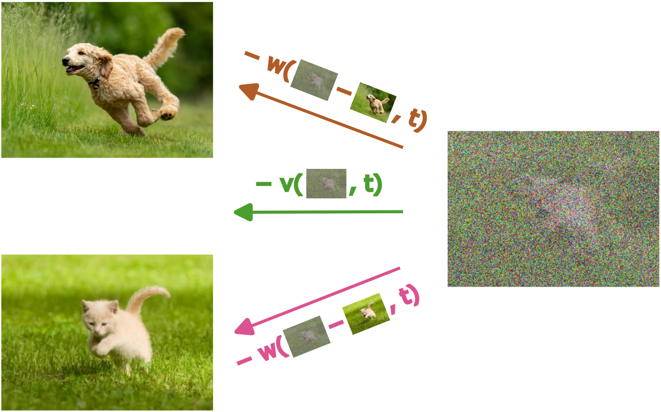
The flow \(v(x, t)\) at a given point \(x\) (shown by the noised image on the right of this figure) is the average of the ‘constituent flows’ from each of the source images. There is a direction from the dog to the noised image, and there is a direction from the cat to the noised image, and the combined flow is the average of these, weighted by the conditional probability of the unnoised image.
Let’s prove Theorem 4.2.
Our aim is to show that that \(v\) and \(\rho\) satisfy the continuity equation. Indeed
\[\begin{align*} \partial_t \rho (x, t) &= \partial_t (\pi * \tau)(x, t) \\ &= \partial_t \int \pi(z) \tau(x - z, t) dz \\ & = \int \pi(z) \partial_t \tau(x - z, t) dz \\ & = - \int \pi(z) \nabla_x \cdot (\tau(x - z, t) w(x-z, t)) dz \qquad\text{by \eqref{eq:continuity_equation}} \\ &= - \nabla_x \cdot \int \pi(z) \tau(x-z, t) w(x-z, t) dz \\ &= -\nabla_x \cdot \left[ v(x, t) \int \pi(z) \tau(x-z, t) dz \right] \qquad\text{by \eqref{eq:explicit_drift_for_convolved}} \\ &= -\nabla \cdot (v(x, t) \cdot (\pi * \tau) (x, t)) \\ &= -\nabla \cdot (v(x, t) \rho (x, t)) \end{align*}\]which is the continuity equation, as required.
To obtain a generative diffusion model, we want to convert this into an algorithm for learning the drift \(v\) by a neural network. One option is to directly parameterize \(v\) as a neural network with parameters \(\theta\), and then use equation \(\eqref{eq:convolved_drift_loss}\) as a loss function and perform stochastic gradient over samples \(z, y\) to learn \(\theta\). An important unspecified aspect is the distribution over time \(t\). Although the true theoretical minimizer of \(\eqref{eq:convolved_drift_loss}\) is independent of the distribution of \(t\), when we have only a neural function approximator, and limited compute budget, the distribution over \(t\) makes a large difference. We look at this and other practical details later on.
It is actually more common to learn a denoiser \(D\), which is conceptually simpler and numerically better conditioned than directly learning the drift \(v\). The denoiser predicts the “unnoised ground truth” value (i.e., at \(t=0\)) given a noisy sample (i.e., as convolved with \(\tau\)).
Gaussian noise
In the case of adding Gaussian noise, the denoiser can be defined as follows.
Given an initial distribution with density function \(\pi(z)\), and \(\sigma \ge 0\), the denoiser is the function \(D(x, \sigma)\) that minimizes
\[\begin{equation} \label{eq:denoiser} \underset{\substack{ z \sim \pi(z) \\ y \sim N(0, \sigma^2) }}{\E} \vert\vert D(y+z, \sigma) - z \vert\vert^2. \end{equation}\]By Exercise 1.5 we can equivalently define
\[\begin{equation*} D(x, \sigma) = \underset{z \vert y+z=x}{\E} z := \frac{ \int \pi(z) n(x-z, \sigma^2) z dz }{ \int \pi(z) n(x-z, \sigma^2) dz } \end{equation*}\]where \(n(\cdot, \sigma^2)\) is the density of a Gaussian with variance \(\sigma^2\).
The following exercise shows how to convert a denoised prediction to a drift.
Recall from Exercise 4.2 that \(w(y, t) = y / t\) is a drift for a Gaussian with variance \(t^2\). By substituting the expressions for \(v(y, t)\) and \(w(x, t)\) into \(\eqref{eq:convolved_drift_loss}\), show that
\[\begin{equation} \label{eq:denoiser_drift_for_adding_gaussian} v(x, t) := \frac{x - D(x, t)}{t} \end{equation}\]is a drift for the family of distributions that arises from adding Gaussian noise with variance \(t^2\) to samples from \(\pi(z)\).
The drift of equation \eqref{eq:denoiser_drift_for_adding_gaussian} is particularly suggestive. For large \(t\), \(D(x, t) \approx \E z\), the unconditional expectation of \(z \sim \pi(z)\), and so \(v(x, t) \approx (x - \E z) / t\) points to the mean of the distribution \(\pi\). As shown in the figure below, at large \(t\) the trajectories are tangent to the line that goes approximately through the origin (the mean of the signed Bernoulli random variable at time \(t=0\)). As we follow this trajectory from large values of \(t\) to smaller values, finer details about the original distribution are resolved, and the trajectories curve towards these; the initial Gaussian noise is gradually and continuously transformed into the distribution \(\pi\) at time \(t=0\). This might be one clue as to why diffusion models perform so well: they are able to incrementally add information about the original distribution, rather than resolving it all at once.
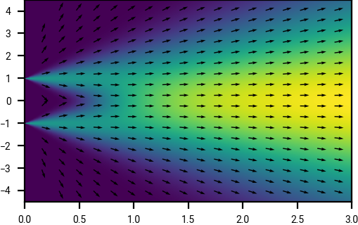
Probability density and drift (velocity) field.
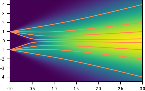
Trajectories at a range of starting points.
Drifts (velocity fields), and example trajectories, for adding Gaussian noise to a signed Bernoulli random variable, as a function of position \(x\) and time \(t\).
To obtain samples, we numerically integrate the drift to obtain trajectories. An important aspect affecting numerical integration error is the curvature of the trajectories.
By using Exercise 3.2, show that the curvature for a trajectory \(\phi(t)\) in the setup of Exercise 4.3 is
\[\begin{equation} \partial_{tt} \phi(t) = - \frac{1}{t} \big( \partial_t + v(\phi(t), t) \cdot \nabla \big) D(\phi(t), t). \end{equation}\]Again, the material derivative (which gives the rate of change along a trajectory) makes an appearance, this time operating on the denoiser \(D\). In particular this implies that if \(D\) is constant along a trajectory, then the curvature is zero, and this allows one-step integration. This idea occurs in consistency diffusion [15]Consistency models
Song, Yang and Dhariwal, Prafulla and Chen, Mark and Sutskever, Ilya
arXiv preprint arXiv:2303.01469, 2023.
Show that when the data distribution \(\pi\) is a discrete distribution, i.e., the support of \(\pi\) consists of a discrete finite set of points \(\mathcal{A} \subset \R^n\), that for Gaussian noise,
\[D(x, \sigma) \rightarrow (1 + o_\sigma(1)) \, \underset{z \in \mathcal{A}}{\text{argmin}} ||z - x||^2\]where \(o_\sigma(1) = o_{\mathcal{A};\, \sigma \rightarrow 0}(1) \rightarrow 0\) as \(\sigma \rightarrow 0\) (this error term can depend on \(\mathcal{A}\), but is independent of \(x\)).
In other words, when \(\sigma\) is small, \(D(x, \sigma) \approx z(x)\) where \(z(x) \in \mathcal{A}\) is the closest point to \(x\) in the support of \(\pi\).
We can visualize the implication of Exercise 4.5.
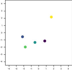
Discrete distribution \(\pi(z)\), in \(n=2\) dimensions, consisting of \(\vert\mathcal{A}\vert = 5\) points.
\(\R^2\) coloured by the final denoised point from following the denoising trajectory backwards from the given time.
Suppose we add Gaussian noise with variance \(t^2\) to a discrete data distribution. Starting at a given \(t\), if we follow the trajectory given by \(\frac{dx}{dt}=v(x,t)\) backwards to \(t=0\), we will up back at one of discrete points. We can colour the space by which point we finish up at, and observe how this partitions the space at a given time. Observe that as \(t \rightarrow 0\), the partitioning of the space increasingly resembles Voronoi cells around \(\mathcal{A}\).
Final remarks
In this section we only looked at deterministic sampling achieved by following a deterministic ODE. If our denoiser is “perfect”, i.e., gives the true conditional expectation of the data distribution, and we follow these trajectories precisely (rather than having numerical integration errors), then we will correctly sample from the data distribution. However this is not always the case, and there are alternative ways of sampling which do not involve following a deterministic ODE, but rather involve following a stochastic differential equation. We will look at this in a later section.
We also only derived the flow for Gaussian noise with variance \(t^2\). More general formulations are possible, and we will also look at these in later sections.
Table of contents
- Home
- Motivating example
- Stochastic processes
- Probability flow
- Deterministic diffusion for Gaussian noise
- Numerical integration
- Reparameterizations of time and space
- Stochastic calculus
- Diffusion via SDEs, and score functions