Reparameterizations of time and space

So far we’ve been looking at adding Gaussian noise with variance \(t^2\) at time \(t\), i.e.,

\[\begin{equation} \label{eq:ddim_or_edm_formulation} X_t \equiv X_0 + t N(0, 1)_{\R^n}. \end{equation}\]

We showed that the function \(v(x, t) = \frac{x - D(x, t)}{t}\), where \(D\) is the denoiser, is a drift for this family of distributions, i.e., following the probability flow ODE \(\frac{dx}{dt} = v(x, t)\) preserves the density of the \(X_t\).

The setup \eqref{eq:ddim_or_edm_formulation} is the DDIM / EDM [11, 10]Denoising diffusion implicit models
Song, Jiaming and Meng, Chenlin and Ermon, Stefano
arXiv preprint arXiv:2010.02502, 2020

Elucidating the design space of diffusion-based generative models
Karras, Tero and Aittala, Miika and Aila, Timo and Laine, Samuli
Advances in Neural Information Processing Systems, 2022 formulation, where the trajectories given by \(v\) at large \(t\) are approximately linear, yielding low numerical error when taking Euler steps. (Sometimes this is referred to as the variance exploding formulation to distinguish it from the variance preserving formulation below, although in [5]Score-based generative modeling through stochastic differential equations
Song, Yang and Sohl-Dickstein, Jascha and Kingma, Diederik P and Kumar, Abhishek and Ermon, Stefano and Poole, Ben
arXiv preprint arXiv:2011.13456, 2020 variance exploding refers to a specific formulation.)

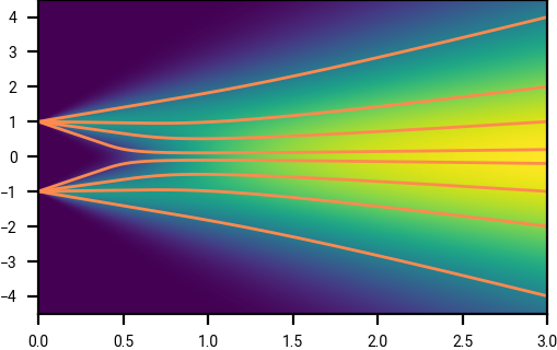
The linear noise schedule that we have so far been using yields approximately linear trajectories at high noise levels, which in turn yields low integration errors when using a first order Euler integrator, as observed in EDM.

Sometimes other formulations are useful.

Variance preserving formulation

When doing numerical computations, as well as feeding quantities into neural networks, it is useful for the vector components to have typical magnitude around \(1\). This avoids numerical representation errors, and aligns with neural networks that are typically configured to learn well when inputs are unit normalized.

For notational convenience, let \(\vert\vert \cdot \vert\vert\) be the norm on \(\R^n\) where \(\vert \vert x \vert \vert_2^2 = \frac{1}{n} \sum_{i=1}^n x_i^2\). (I.e., \(\vert\vert \cdot \vert\vert\) is the usual Euclidean norm, normalized by \(1/\sqrt{n}\).) Under this norm, this says that we want most vectors that we work with to have magnitude around \(1\).

In the EDM / DDIM formulation \eqref{eq:ddim_or_edm_formulation}, the noisy input \(X_t\) is renormalized before feeding into the neural network. However, we can also work with a stochastic process where the noised values are already normalized. Given an unnormalized target distribution \(Z\) for \(t=0\), this can be achieved for \(X_t\) by defining

\[\begin{equation} \label{eq:unit_normalized_Xt} X_t \equiv \frac{Z + t N(0, 1)_{\R^n}}{\sqrt{\sigma_\text{data}^2 + t^2}} \end{equation}\]

where \(\sigma_\text{data} := ( \E || Z ||^2 )^{1/2}\). This corresponds to a rescaling of space \(y = \alpha(t) x\) for some function \(\alpha(t)\).

Exercise 6.1: Renormalized has unit variance

Show that \(\E \vert\vert X_t \vert\vert^2 = 1\) where \(X_t\) is defined in \eqref{eq:unit_normalized_Xt}.

It can also be useful to reparameterize time.

Unit time range

For reasons of analysis and numerics, it is also sometimes useful for the range of time to be \([0, 1]\) with \(X_1\) an exact Gaussian, rather than \([0, T]\) where \(T \gg 1\) is a sufficiently large value such that \(X_T\) is approximately Gaussian.

We can achieve this via a monotonic reparameterization of time \(s=s(t)\) where \(s(0)=0\) and \(s(\infty)=1\).

Different space and time scalings are in some sense all equivalent (the underlying spaces are just transformations of each other); in practical implementations, the inputs to the neural network will be scaled to have norm 1, whether this happens “within the diffusion process” \(X_t\), or on the “neural network side”. There are a couple of caveats:

Adjusting the scaling of the coordinates or time can affect the curvature of trajectories, which has an effect when using a first-order Euler method to integrate. There are ways of counteracting this, but it requires consideration; naïvely using a space with non-trivial curvature can significantly affect the performance when using the wrong numerical integration approach.
The numerics (due to limited floating point precision) are affected, and this can be a desired or undesired effect effect.

The variance preserving formulation can be easier to debug when implementing it, because vectors with the incorrect norm are more obvious (and less upscaling and downscaling of vectors is required), but it does require more complexity elsewhere, and the trajectory curvature has to be considered when using first-order methods.

How do the drift terms change under reparameterizations of time and space?

Exercise 6.2: Reparameterizations of time and space

In the following, \((Y_s)_{s \in I}\) is a reparameterization of \((X_t)_{t \in I'}\) for time intervals \(I, I' \subset \R\), and \(v\) and \(w\) are drifts for \(X_t\) and \(Y_s\) respectively, i.e., obeying \(\frac{d X_t}{dt} = v(X_t, t)\) and \(\frac{d Y_s}{ds} = w(Y_s, s)\).

Let \(s=s(t)\) be a reparameterization of time with inverse \(t(s)\), so \(Y_s = X_{t(s)}\). Show that
\[w(x, s) = \frac{dt}{ds} v(x, t(s)).\]
Use this, and the result of Exercise 4.2 to deduce that a drift for a Gaussian with standard deviation \(\sigma(s)\) at time \(s\) is
\[\frac{\sigma'(s)}{\sigma(s)} x.\]
Let \(Y_t = \alpha(t) X_t\) be rescaled coordinates for some time-dependent rescaling function \(\alpha(t)\). Show that
\[w(y, t) = \frac{\alpha'(t)}{\alpha(t)} y + \alpha(t) v(y / \alpha(t), t).\]
What is the time-indexed probability density for \(Y_t\) in terms of that for \(X_t\)?
Let \(s=s(t)\) be a reparameterization of time with inverse \(t=t(s)\), and \(y=\alpha(s)x\) a rescaling of coordinates by \(\alpha(s)\). Show that
\[w(y, s) = \frac{\alpha'(s)}{\alpha(s)} y + \alpha(s) \frac{dt}{ds} v(y/\alpha(s), t(s)).\]
What is the time-indexed probability density for \(Y_t\) in terms of that for \(X_t\)?

Confirm also that this formula yields \((\sigma'(s) / \sigma(s)) y\) for the drift of a Gaussian with standard deviation \(\sigma(s)\) at time \(s\), independent of \(\alpha(s)\).

Exercise 6.3: Drift for general scaling and noise levels

Exercise 4.3 gave a drift for \(X_t = Z + t N(0, 1)_{\R^n}\) in terms of the denoiser \(D(x, \sigma)\). Suppose instead that

\[X_s \equiv \alpha(s) Z + \sigma(s) N(0, 1)_{\R^n}\]

where \(\alpha(s) \in \R\) is an arbitrary scaling, and \(\sigma(s)\) is the noise level. Apply the coordinates rescaling result of Exercise 6.2 to the result of Exercise 4.3 to show that the drift is

\[\begin{equation} \label{eq:denoiser_scaled} \frac{\dot{\sigma}(s)}{\sigma(s)} y + \left( \dot{\alpha}(s) - \frac{\alpha(s) \dot{\sigma}(s)}{\sigma(s)} \right) D \left( \frac{y}{\alpha(s)}, \frac{\sigma(s)}{\alpha(s)} \right). \end{equation}\]

The quantity \(\alpha(s) / \sigma(s)\) is known as the signal-to-noise ratio (SNR), and acts like a “sufficient statistic”. The reciprocal quantity \(\sigma(s) / \alpha(s)\) is sometimes the inverse noise-to-signal ratio (iSNR).

Exercise 6.4: Reparameterizations and numerics

Recall Exercise 5.5 on the numerics of integration and floating point precision. Is it possible to find a schedule \(\alpha(s)\) and \(\sigma(s)\) such that it is safe to do integration in reduced precision, or is this never possible?

Exercise 6.5: Integration error under reparameterizations

Let \(v(x, t) = x/t\), whose integral yields trajectories \(\Phi(t; x_0, t_0) = \frac{t}{t_0} x_0\).

Euler integration across timesteps \(t_0 > t_1 > \cdots > t_N = 0\) gives the sequence of points

\[x_{i+1} = x_i + (t_{i+1} - t_i) v(x_i, t_i).\]

What is the curvature (as per Exercise 3.2) of the trajectories \(\phi(t) = \Phi(t; x_0, t_0)\) for fixed \(x_0, t_0\)?
Show that no matter what the time steps \(t_i\), the final value of \(x_N\) is zero.

Now consider the time reparameterization where \(s(t) = t^2\), which has drift term \(w(x, s)\) (as per Exercise 6.2).

What is \(w(x, s)\)? What do the trajectories look like?
If we integrate across time steps \(s_i = 1 - i/N\), what is the value of \(x_{i+1}\) in terms of \(x_i\)?
What is the final integration error \(x_N\)?

Rectified flow

We can extend some of our results from calculating the drift of a convolved distribution, in particular Gaussians, to more general time-indexed families of distributions. One such example is rectified flow [19]Flow straight and fast: Learning to generate and transfer data with rectified flow
Liu, Xingchao and Gong, Chengyue and Liu, Qiang
arXiv preprint arXiv:2209.03003, 2022, which interpolates between two distributions.

Theorem 6.1: Rectified flow

Let \(X_0\), \(X_1\) be two independent random variables taking values in \(\R^n\). For \(0 \le t \le 1\) let \(X_t = (1-t) X_0 + t X_1\), and let \(\tau(x, t)\) be the probability density of \(x \sim X_t\).

Then the minimizer \(v(x, t)\) of the following is a drift for \(\tau(x, t)\).

\[\begin{equation} \underset{\substack{ x_0 \sim X_0 \\ x_1 \sim X_1 }}{\E} || (x_1 - x_0) - v((1-t) x_0 + t x_1, t) ||^2. \end{equation}\]

Theorem 6.1 can be derived from Theorem 4.2 through an appropriate rescaling of coordinates. In some sense, it is “only” a rescaling of the diffusion setup, however, this is a canonical scaling that enjoys certain properties, and in particular has low curvature when doing Euler integration.

Exercise 6.6: Rectified flow is canonical for minimizing curvature over \(t=[0, 1]\)

Let \(X_t = \alpha(t) X_0 + \sigma(t) N(0, 1)\) for \(0 \le t \le 1\). Show that the only functions \(\alpha(t)\) and \(\sigma(t)\) that result in straight trajectories for all \(X_0\) that are deterministic are

\[\alpha(t) = 1 - t, \qquad \sigma(t) = t,\]

i.e., rectified flow. (In general, \(X_0\) is not deterministic, and so the trajectories cannot be straight, but we have “removed the curvature” that is due to just the diffusion space itself.)

There are even more general forms of Theorem 6.1, for example flow matching [20]Flow matching for generative modeling
Lipman, Yaron and Chen, Ricky TQ and Ben-Hamu, Heli and Nickel, Maximilian and Le, Matt
arXiv preprint arXiv:2210.02747, 2022 which in turn has connections to things like optimal transport (not covered here).