8. Diffusion via SDEs, and score functions
So far the perspective has been:
- The forward noising process is “one shot” (adding noise for time \(t\) to the unnoised distribution).
- The backwards sampling process follows a deterministic ODE.
Now we have the tools of stochastic processes and stochastic calculus, and we can apply these to get a new perspective on diffusion, at least in the case of adding Gaussian noise. In this section, we will take the perspective of:
- The forward noising process incrementally adds noise, following a stochastic process.
- The backwards sampling process can arise by following a stochastic differential equation (SDE), which has the same marginal but different joint distribution and properties.
We’ve deferred this approach until this section, since it requires the more advanced machinery of stochastic calculus, and many of the fundamental diffusion results can be derived without it. But the language and framework of SDEs is now standard in the diffusion literature, so it is useful to be familiar with it. It also allows results, such as determining variational bounds, which aren’t possible otherwise.
The forward process
Recall from the section on Stochastic processes that Brownian motion, corresponding to the stochastic process with SDE \(dX_t = dW_t\), yields the marginal distribution \(X_t \equiv X_0 + N(0, t)\). There is a more general form of this.
Let \(\alpha, \sigma : [0, \infty) \rightarrow [0, \infty)\) with \(\alpha(0)=1\) and \(\sigma(0)=0\), and let \(Z\) be an arbitrary random variable. By working from first principles as in Exercise 7.3 or otherwise, show that the SDE that yields the stochastic process \((X_t)_{t \ge 0}\) with \(X_0 \equiv Z\) and with marginal distribution
\[\begin{equation} \label{eq:marginal_with_alpha_and_sigma} X_t \equiv \alpha(t) Z + N(0, \sigma(t)^2) \end{equation}\]is
\[\begin{equation} \label{eq:sde_for_marginals_alpha_and_sigma} dX_t = \frac{\dot{\alpha}(t)}{\alpha(t)} X_t ~ dt + \sqrt{ 2 \sigma(t) \dot{\sigma}(t) - 2\frac{\dot{\alpha}(t)}{\alpha(t)} \sigma(t)^2 } \, dW_t \end{equation}\]where \(\dot{\alpha} = \frac{d \alpha}{d t}\) and \(\dot{\sigma} = \frac{d \sigma}{d t}\).
Observe this only exists when the expression inside the square root is non-negative. What does this constraint correspond to?
The backwards process
We are going to derive a stochastic differential equation which when integrated backwards, yields the same marginal distributions \(X_t\) as in the forward process. In fact, since an ODE is a special case of an SDE, we have already done this in Exercise 4.3 (for Gaussian noise \(N(0, t^2)\)) and in Exercise 6.3 (for more general noise \eqref{eq:marginal_with_alpha_and_sigma}).
We already saw in Exercise 4.1 that there are multiple ODEs which all yield the same marginal distributionss, and if we allow ourselves the freedom of SDEs, there are even more. The different SDEs correspond to “injecting” different amounts of noise during the backwards process, and although they theoretically yield the same distribution, one may be a more practically preferred choice when combined with an imperfect denoiser.
Fokker-Planck equation
When looking at deterministic ODEs in the context of probability flow, the key result that allowed us to go between a time-indexed family of densities \(\rho(x, t)\) and an ODE was the continuity equation Theorem 3.3.
This can be generalized to the density which arises from an SDE, and is known as the Fokker-Planck equation.
Let \(X_t\) be a 1-dimensional stochastic process with drift \(v(x, t)\) and diffusion coefficient \(\kappa(x, t)\), i.e., described by
\[dX_t = v(X_t, t) \, dt + \kappa(X_t, t) \, dW_t.\]Let \(\rho(x, t)\) be the probability density function of \(X_t\). The time-derivative of \(\rho\) obeys
\[\begin{equation} \label{eq:fokker_planck_1d} \frac{\partial \rho}{\partial t} = - \frac{\partial}{\partial x} ( \rho v ) + \frac{1}{2} \frac{\partial^2}{\partial x^2} ( \kappa^2 \rho ). \end{equation}\]Observe that if the diffusion coefficient \(\kappa \equiv 0\), then \eqref{eq:fokker_planck_1d} reduces to the continuity equation seen in Theorem 3.3. This is expected: an SDE with \(\kappa \equiv 0\) is just an ODE.
The proof mirrors that of Theorem 3.3 and of Lemma 7.1.
Let \(F : \R \rightarrow \R\) be continuous with continuous first and second derivatives, and be compactly supported, i.e., vanishing at infinity. (\(F\) is a test function.)
Consider the map
\[\begin{equation} \label{eq:t_map_in_fp_proof} t \mapsto \E F(X_t). \end{equation}\]By the definition of expectation, this equals \(\int \rho(x, t) F(x) dx\). The derivative of this with respect to \(t\) is
\[\begin{equation} \label{eq:defn_deriv_proof_fp} \int \partial_t \rho (x, t) F(x) dx. \end{equation}\]But also, by Taylor expansion of \(F\),
\[F(X_{t+dt}) = F(X_t) + dX_t F_x(X_t) + \frac{1}{2} dX_t^2 F_{xx} (X_t) + O(|dX_t|^3).\]Observe that \(\E dX_t = v(X_t, t) dt\) and \(\E dX_t^2 = \kappa(X_t, t)^2 dt\), and so taking expectations of this Taylor expansion yields
\[\E F(X_{t+dt}) = \E F(X_t) + \E v(X_t, t) F_x (X_t) dt + \frac{1}{2} \E \kappa(X_t, t)^2 F_{xx} (X_t) dt + o(dt).\]Thus by taking the limit \(dt \rightarrow 0\), we have
\[\begin{align*} \frac{d}{d t} \E F(X_t) &= \E v(X_t, t) F_x (X_t) + \frac{1}{2} \E \kappa(X_t, t)^2 F_{xx} (X_t) \\ &= \int \rho(x, t) v(x, t) F_x(x) dx + \frac{1}{2} \int \rho(x, t) \kappa(x, t)^2 F_{xx}(x) dx \\ &= -\int \frac{\partial}{\partial x} \big( \rho(x, t) v(x, t) \big) F(x) dx + \int \frac{1}{2} \frac{\partial^2}{\partial x^2} \big( \rho(x, t) \kappa(x, t)^2 \big) F(x) dx \\ &= \int \left( - \frac{\partial}{\partial x} \big( \rho(x, t) v(x, t) \big) + \frac{1}{2} \frac{\partial^2}{\partial x^2} \big( \rho(x, t) \kappa(x, t)^2 \big) \right) F(x) dx \end{align*}\]where we have used integration by parts. Comparing this expression with \eqref{eq:defn_deriv_proof_fp}, and using the fact that \(F\) was arbitrary, we obtain \eqref{eq:fokker_planck_1d}.
Generalize Theorem 8.1 to \(n\) dimensions. Namely, show that if \(X_t\) is a stochastic process described by
\[dX_t = v(X_t, t) \, dt + \kappa(X_t, t) \, dW_t\]where \(v(x, t) \in \R^n\) and \(\kappa(x, t) \in \R^{n \times n}\), then the time-derivative of the probability density function \(\rho(x, t)\) of \(X_t\) obeys
\[\begin{equation} \label{eq:fokker_planck} \frac{\partial \rho}{\partial t} = - \sum_i \frac{\partial}{\partial x_i} ( \rho v )_i + \frac{1}{2} \sum_{i, j} \frac{\partial^2}{\partial x_i \partial x_j} ( \kappa \kappa^T \rho )_{ij}. \end{equation}\]Converting an SDE to an ODE
As used in [5]Score-based generative modeling through stochastic differential equations
Song, Yang and Sohl-Dickstein, Jascha and Kingma, Diederik P and Kumar, Abhishek and Ermon, Stefano and Poole, Ben
arXiv preprint arXiv:2011.13456, 2020, the Fokker-Planck equations \eqref{eq:fokker_planck_1d} and \eqref{eq:fokker_planck} imply that we can switch between an SDE, and an ODE (the probability-flow ODE), with the same marginal distributions. Let \(\rho(x, t)\) be the density of the stochastic process defined by the (forward-time) SDE \eqref{eq:forward_time_sde}, where we restrict the diffusion coefficient \(\kappa(t)\) to only depend on \(t\). Then provided that the stochastic processes have the same marginals at some \(t_0\), it can be shown that the stochastic process (in fact, a deterministic probability flow) defined by the ODE \eqref{eq:forward_time_sde_to_ode} has the same marginal distribution, as shown in the exercise below.
By using the Fokker-Planck equation \eqref{eq:fokker_planck_1d}, \eqref{eq:fokker_planck}, show the stochastic process \(X_t\) given by the (forward-time) SDE \eqref{eq:forward_time_sde} and the ODE given by \eqref{eq:forward_time_sde_to_ode} have the same marginal distributions.
The term reverse-time SDE indicates that the SDE should be integrated backwards. This ability to go between an SDE and an ODE with the same marginals allows us to convert between forward-time and reverse-time SDEs with the same marginals, via an intermediate ODE. Applying this result twice (to get an intermediate ODE) gives a reverse-time SDE with the same marginals as the forward-time SDE \eqref{eq:forward_time_sde} and an arbitrary diffusion coefficient \(\tilde{\kappa}(t)\):
\[\begin{equation} \label{eq:reverse_time_sde} dY_t = \left( v(Y_t, t) - \frac{1}{2} (\kappa(t)^2 + \tilde{\kappa}(t)^2) ~ \nabla \log \rho(Y_t, t) \right) dt + \tilde{\kappa}(t) dW_t \end{equation}\]In particular, by taking \(\tilde{\kappa} = \kappa\), the following reverse-time SDE has the same diffusion coefficient and yields the same overall distribution on stochastic processes as the forward-time SDE \eqref{eq:forward_time_sde}.
\[\begin{equation} dY_t = \left( v(Y_t, t) - \kappa(t)^2 ~ \nabla \log \rho(Y_t, t) \right) dt + \kappa(t) dW_t \end{equation}\]Applying this to diffusion
In particular, applying the SDE to ODE conversion formula \eqref{eq:forward_time_sde_to_ode} to \eqref{eq:sde_for_marginals_alpha_and_sigma} yields the following ODE, that if integrated (backwards or forwards), will yield the same set of marginal distributions as in the forwards noising process.
\[\begin{equation} \label{eq:score_ode_for_alpha_and_sigma} \frac{dY_t}{dt} = \frac{\dot{\alpha}(t)}{\alpha(t)} Y_t + \left ( \frac{\dot{\alpha}(t)}{\alpha(t)} \sigma(t)^2 - \sigma(t) \dot{\sigma}(t) \right ) \nabla \log \rho(Y_t, t) \end{equation}\]I.e., this is an ODE that gives the marginal distributions \eqref{eq:marginal_with_alpha_and_sigma}. Thus this almost allows us to sample, except that this ODE has a mysterious term \(\nabla \log \rho\) in it. What is this? How can we estimate it? How does it relate to the previous ODE we derived involving the denoiser term (see Exercise 6.3)?
The score function
The term \(\nabla \log \rho\) is known as the score function.
Given a probability density function \(\pi(x)\) over a vector space \(x \in \R^n\), the (Stein) score function [21, 22]A kernel test of goodness of fit
Chwialkowski, Kacper and Strathmann, Heiko and Gretton, Arthur
International conference on machine learning, 2016
A kernelized Stein discrepancy for goodness-of-fit tests
Liu, Qiang and Lee, Jason and Jordan, Michael
International conference on machine learning, 2016 is the gradient of the log of the probability density function,
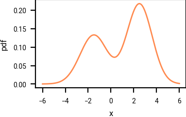
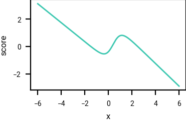
Example of a probability density function, and its corresponding score function.
There is a lot that can be said about the score function, and we don’t cover it extensively here, except to remark that the score function is invariant to the normalization constant of the density, since for a constant \(C \in \R\), \(\nabla \log (C \pi(x)) = \nabla \log \pi(x)\), and
that estimating an unnormalized density (for example, through machine learning methods) is often easier than estimating the normalized density of a distribution.
For a larger overview of the score function, see [3, 23]Generative Modeling by Estimating Gradients of the Data Distribution
Song, Yang
https://yang-song.net/blog/2021/score/
How to train your energy-based models
Song, Yang and Kingma, Diederik P
arXiv preprint arXiv:2101.03288, 2021.
Does every score function \(s : \R^n \rightarrow \R^n\) correspond to a distribution? In one dimension \(n=1\), we can build an ansatz probability density via
\[\tilde{\pi}(x) = \exp \left( \int_0^x s(y) dy \right)\]and define \(\pi(x) = \tilde{\pi}(x) / Z\) where \(Z = \int \tilde{\pi}(y) dy\). Provided that \(Z\) exists, it is easy to see that the score function of \(\pi\) is equal to \(s(x)\). However, \(Z\) need not exist; a simple counterexample is \(s(x) = -\log(1+|x|)\). In higher dimensions, we also require that the score function is conservative, which means it is the gradient of a function \(f : \R^n \rightarrow \R\).
The score function \eqref{eq:score_function} is only defined when \(\pi(z)\) is non-zero and everywhere differentiable. In particular, discrete distributions (such as the distribution over images with discretized pixel values) do not have a score function. In diffusion, we convolve the discrete distribution with a Gaussian, which makes it everywhere smooth. However, if the variance of the Gaussian is low, the resulting distribution may still have somewhat isolated islands of probability, and although the score function exists, deriving the density from it is also ill-conditioned, and approaches for sampling such as Langevin dynamics (see below) are similarly ill-conditioned. Indeed, generative diffusion models, where a data distribution is noised with an increasingly high-variance Gaussian to connect these islands of probability, were initially motivated to make Langevin dynamics work.
Learning the score function
It turns out that we can estimate and learn the score function of a density \(\rho\), provided we can sample from \(\rho\). The next lemma says that the explicit score-matching loss, which is the L2 loss on approximating the score function with another function \(s(x)\), can be rewritten to an expression that does not explicitly involve the density \(\rho\), plus a constant independent of \(s\), as shown in [24]Estimation of non-normalized statistical models by score matching.
Hyvärinen, Aapo and Dayan, Peter
Journal of Machine Learning Research, 2005
Let \(R = \R^n\) be a sample space and let \(\rho : R \rightarrow \R\) be a density function. Then there exists a constant \(c\) such that for all \(s : R \rightarrow R\),
\[\begin{equation} \underbrace{\frac{1}{2} \underset{x \sim \rho(x)}{\E} || s(x) - \nabla \log \rho(x) ||^2}_\text{explicit score-matching loss} = \underbrace{\frac{1}{2} \underset{x \sim \rho(x)}{\E} \big \{ || s(x) ||^2 + 2 \nabla \cdot s(x) \big \}}_\text{implicit score-matching loss} + c. \end{equation}\]The proof is straightforward and follows using integration-by-parts. Expanding out the definition of expectation and applying integration by parts yields
\[\begin{align*} \frac{1}{2} \underset{x \sim \rho(x)}{\E} || s(x) - \nabla \log \rho(x) ||^2 &= \frac{1}{2} \int \rho(x) || s(x) - \nabla \log \rho(x) ||^2 \, dx \\ &= \frac{1}{2} \int \rho(x) \left( || s(x) ||^2 - 2 s(x) \cdot \nabla \log \rho(x) + || \nabla \log \rho(x) ||^2 \right) dx \\ &= \frac{1}{2} \int \rho(x) \left( || s(x) ||^2 + 2 \nabla \cdot s(x) + || \nabla \log \rho(x) ||^2 \right) dx \\ &= \frac{1}{2} \underset{x \sim \rho(x)}{\E} \big \{ || s(x) ||^2 + 2 \nabla \cdot s(x) + || \nabla \log \rho(x) ||^2 \big \} \end{align*}\]where the last term \(c := \frac{1}{2} \underset{x \sim \rho(x)}{\E} \vert\vert \nabla \log \rho(x) \vert\vert^2\) is independent of \(s\) as required.
The implicit score-matching loss in the above lemma may still not be tractable to calculate, since it involves the term \(\nabla \cdot s\), and this prevents us from using it to learn the score function. However, the next lemma says that we can write the (explicit) score-matching loss as an expectation over a conditional distribution, plus a constant independent of \(s\). For many distributions, for example when \(x\) is equal to \(z\) plus Gaussian noise, the score function of this conditional distribution is tractable, and this allows us to learn a score function. This lemma is somewhat analogous to Theorem 4.2, and is given in [25]A connection between score matching and denoising autoencoders
Vincent, Pascal
Neural computation, 2011.
Let \(Z\) and \(X\) be (non-independent) random variables on sample space \(R\), with density functions \(\pi\) and \(\rho\) respectively, and write \(\rho(x \vert z)\) for the conditional density of \(x \sim X\) conditioned on \(Z=z\). There exists a constant \(c'\) such that for all \(s : R \rightarrow R\),
\[\begin{equation} \label{eq:denoising_score_matching_loss} \underbrace{\frac{1}{2} \underset{x \sim \rho(x)}{\E} || s(x) - \nabla \log \rho(x) ||^2 }_\text{explicit score-matching loss} = \underbrace{\frac{1}{2} \underset{\substack{z \sim \pi(z) \\ x \sim \rho(x | z)}}{\E} || s(x) - \nabla \log \rho(x | z) ||^2}_\text{denoising score-matching loss} + c'. \end{equation}\]This follows from the score matching result. Indeed, the expectation on the right hand side of \eqref{eq:denoising_score_matching_loss} is
\[\begin{align*} \underset{\substack{z \sim \pi(z) \\ x \sim \rho(x | z)}}{\E} || s(x) - \nabla \log \rho(x | z) ||^2 &= \underset{z \sim \pi(z)}{\E} \underset{x \sim \rho(x | z)}{\E} || s(x) - \nabla \log \rho(x | z) ||^2 \\ &= \underset{z \sim \pi(z)}{\E} \underset{x \sim \rho(x | z)}{\E} \big \{ || s(x) ||^2 + 2 \nabla \cdot s(x) \big \} + c\\ &= \underset{x \sim \rho(x)}{\E} \big \{ || s(x) ||^2 + 2 \nabla \cdot s(x) \big \} + c \\ &= \underset{\substack{z \sim \pi(z)}}{\E} || s(x) - \nabla \log \rho(x) ||^2 + c \end{align*}\]as required.
Applying this to diffusion
Let’s now re-derive the probability flow ODE for diffusion sampling, using the tools of this section.
For the diffusion process with SDE \eqref{eq:sde_for_marginals_alpha_and_sigma}, where \(\rho(x, t \vert z)\) is the density of \(N(\alpha(t) z, \sigma(t)^2)\), show that
\[\nabla \log \rho(x, t | z) = \frac{\alpha(t) z - x}{\sigma(t)^2}.\]Per Definition 4.3 the denoiser \(D\) is the function that takes a noised sample, and predicts the original unnoised sample. We can generalize this to the current setting by defining \(D : R \times \R \rightarrow R\) to be the minimizer of
\[\underset{\substack{ z \sim \pi(z) \\ y \sim N(0, \sigma(t)^2) }}{\E} ||D(\alpha(t)z + y, \sigma(t)) - z||^2\](this is well-defined if \(\sigma(t)\) is strictly monotonic in \(t\) and hence invertible). If \(s(x, t)\) is the minimizer of the denoising score-matching loss \eqref{eq:denoising_score_matching_loss} then
\[\begin{align*} s(x, t) = \frac{\alpha(t) D(x, \sigma(t)) - x}{\sigma(t)^2}. \end{align*}\]Use \eqref{eq:score_ode_for_alpha_and_sigma} to re-derive Exercise 6.3, namely, that the drift for a diffusion process with scaling \(\alpha(t)\) and noise level \(\sigma(t)\) is
\[v(x, t) = \frac{\dot{\sigma}(t)}{\sigma(s)} x + \left( \dot{\alpha}(t) - \frac{\alpha(s) \dot{\sigma}(t)}{\sigma(t)} \right) D \left( \frac{x}{\alpha(t)}, \frac{\sigma(t)}{\alpha(t)} \right).\]In particular, this gives an alternative approach (using the tools of stochastic calculus) to the result of Exercise 4.3: for \(\alpha(s) = 1\) and \(\sigma(t) = t\), this reduces to the ODE
\[\frac{dX_t}{dt} = v(x, t) = \frac{1}{t}x - \frac{1}{t} D(x, t) = \frac{x - D(x, t)}{t}\]as expected.
Conclusion
We have rederived some of the fundamental results of diffusion for deterministic sampling using stochastic calculus, in particular the Fokker-Planck equation, and briefly introduced the score function. There are many directions to explore once one has a stochastic calculus approach to diffusion.
As remarked earlier, there are many SDEs that yield the same set of marginals when integrated backwards. These correspond to adding different amounts of noise during sampling. This is related to something called Langevin dynamics. The Elucidating Diffusion Models paper [10]Elucidating the design space of diffusion-based generative models
Karras, Tero and Aittala, Miika and Aila, Timo and Laine, Samuli
Advances in Neural Information Processing Systems, 2022 implements Langevin dynamics by adding additional noise during the sampling procedure at a subset of the time steps, and then taking larger integration steps to compensate for this added noise.
For a much larger overview of the score function and Langevin dynamics, see the excellent Generative Modeling by Estimating Gradients of the Data Distribution.
Table of contents
- Home
- Motivating example
- Stochastic processes
- Probability flow
- Deterministic diffusion for Gaussian noise
- Numerical integration
- Reparameterizations of time and space
- Stochastic calculus
- Diffusion via SDEs, and score functions