2. Stochastic processes
The example on the previous page defined random variables \(X_t\) for times \(t \in I = [0, +\infty)\) in a couple of different ways.
- For the “forward noising process”, we defined \(X_t = X_0 + N(0, t^2)\), where \(X_0\) had uniform distribution over \(\{-1, +1\}\).
- For the “backwards process”, we defined \(X_t\) by integrating a given ODE backwards from a sample \(X_T \equiv N(0, T^2)\).
We didn’t specify the joint dependence structure for the \(X_t\) at different \(t\), and in fact there are multiple possibilities. For example, for \(s \ne t\), we might have \(X_s = X_0 + A\) and \(X_t = X_0 + B\) where \(A \equiv N(0, s^2)\) and \(B \equiv N(0, t^2)\) are two independent Gaussian random variables. Or for \(s < t\) we could set \(X_t = X_s + N(0, t^2 - s^2)\). Both of these give rise to the same marginal distributions, but have different joint dependence structure.
Stochastic processes
A set of random variables \((X_t)_{t \in I}\) indexed by times \(I \subset \R\) is known as a stochastic process. The \(X_t\) for different \(t\) might or might not be independent, and \(I\) can be a discrete or a continuous subset of \(R\). If \(I\) is continuous, then typically it is an interval (i.e., a connected subset of the reals).
-
Define \(X_t = 0\) for all \(t \in \R\). This is a very simple stochastic process over the times \(I=\R\), where each random variable \(X_t\) is deterministic, and independent of all other random variables.
-
Let \(X_1 \sim N(0, 1)\) be a Gaussian, and let \(X_t = t X_1\). Then \((X_t)_{t \in [0, 1]}\) is a stochastic process over the time interval \([0, 1]\), where \(X_s\) is determined by \(X_t\) for all \(s\) provided \(t > 0\).
-
\((X_t)_{t \in I}\) defined by \eqref{eq:example_discrete_brownian} below is a stochastic process over the discrete set of times \(I = \{0, 1/k, 2/k, \ldots\}\).
Brownian motion
Let’s start with an example. Define the following sequence of random variables \(X_i\) for \(i=0, 1, 2, \ldots\)
\[\begin{equation} \label{eq:example_discrete_brownian} X_0 = 0 \qquad X_i = X_{i-1} + N(0, 1) \end{equation}\]What is the distribution of \(X_i\) as defined in \(\eqref{eq:example_discrete_brownian}\)?
We have a collection of random variables \(X_i\), each of which is distributed as \(X_i \equiv N(0, i)\), and are not independent of each other. In this example, the random variables are scalar-valued, but similar processes can be defined in higher dimensions.
The stochastic process given by \(\eqref{eq:example_discrete_brownian}\) is an example of (discrete) Brownian motion. This is a very important set of stochastic processes, almost being the canonical diffusion process. Brownian motion (or strictly speaking a Wiener process) is defined as a stochastic process obeying the following.
Let \(I \subset [0, \infty)\) be a set of times containing \(0\). A (one dimensional) Wiener process is a stochastic process \((X_t)_{t \in I}\) obeying the following.
- \(X_0=0\).
- With probability 1, the map \(t \mapsto X_t\) is a continuous function on \(I\).
- For every \(0 \le t_- < t_+\), the increment \(X_{t_+} - X_{t_-}\) has the distribution \(N(0, t_+ - t_-)\). (In particular, \(X_t \equiv N(0, t)\).)
- For every set of times \(t_0 \le t_1 \le \cdots \le t_n\) in \(I\), the increments \(X_{t_i} - X_{t_{i-1}}\) for \(i=1, \ldots, n\) are jointly independent.
Technically, Brownian motion refers to a certain construction of a stochastic process, and Wiener process refers to any stochastic process obeying the set of rules above, i.e., the latter is a model for the former. However the stochastic process obeying these rules is unique [13]Brownian motion and Dyson Brownian motion
Tao, Terence
https://terrytao.wordpress.com/2010/01/18/254a-notes-3b-brownian-motion-and-dyson-brownian-motion, and so we abuse notation and use the two terms somewhat interchangeably here.
-
Verify that the process given by \(\eqref{eq:example_discrete_brownian}\) is a Wiener process.
-
Given an arbitrary discrete set of times \(0 = t_0 < t_1 < t_2 < \cdots\), how can we modify this construction to give a Wiener process over \(I=\{t_0, t_1, t_2, \ldots\}\)?
Amazingly, we can also construct Wiener processes over continuous time segments.
There exists a Wiener process \((X_t)_{t \in [0, +\infty)}\) over all \(t \ge 0\).
We sketch a proof of Proposition 2.2 in the following exercise.
The strategy is to recursively build the process on dyadic rationals at all levels.
-
Let \(A \equiv N(0, 1)\) and \(B \equiv N(0, 1/4)\) be independent. Show that \(A/2 + B\) and \(A/2 - B\) are independent, and are distributed as \(N(0, 1/2)\).
-
By Exercise 2.2 there exists a Wiener process \((X_t)_{t \in \N}\) on the natural numbers. Deduce that the extension of this on \(\frac{1}{2} \N = \{\frac{1}{2}n : n \in \N\}\) by setting
\[X_{t + \frac{1}{2}} = (X_t + X_{t+1}) / 2 + N(0, 1/4)\]is also a Wiener process.
-
By recursively repeating this operation, show that we can construct a Wiener process on the set of times \(2^{-k} \N\) for any \(k=0, 1, 2, \ldots\).
The remainder of the proof is slightly (but not by much) more technical, and for details see [13]Brownian motion and Dyson Brownian motion
Tao, Terence
https://terrytao.wordpress.com/2010/01/18/254a-notes-3b-brownian-motion-and-dyson-brownian-motion. Since each extended Wiener process is consistent with the previous one, it is possible to take the limit of this repeated operation to obtain a Wiener process over the dyadic rationals, which are dense in \([0, +\infty)\). By the law of large numbers, the map \(t \mapsto X_t\) is almost surely Hölder continuous, and thus the Wiener process over the dyadic rationals can be extended to a continuous function on \([0, +\infty)\).
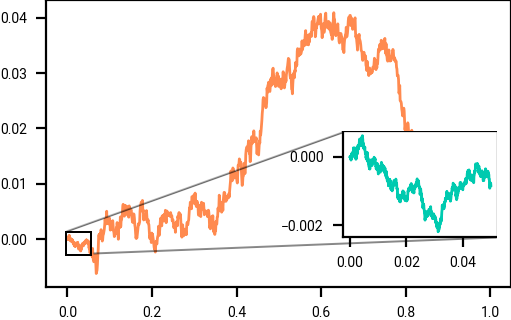
Brownian motion is self-similar: if you zoom in, it looks the same. Mathematically, if you scale the time-axis by \(s > 0\) and the spatial axis by \(\sqrt{s}\), then the distribution is identical.
The marginal distribution of a Wiener process at time \(t\) is \(N(0, t)\). We can also construct a Wiener process where \(X_0\) is a random variable with an arbitrary distribution. The resulting marginal distributions of \(X_t\) are then the convolution of the distribution of \(X_0\) and \(N(0, t)\), rather than purely \(N(0, t)\); the original distribution has had noise added.
Relating this to diffusion models
The example on the previous page almost fits this setup, except that the amount of noise added at time \(t\) was \(N(0, t^2)\) rather than \(N(0, t)\). We will develop tools of stochastic calculus in a later section to handle this setup. For now, we do not yet need the full power of stochastic calculus for deriving diffusion results.
We can visualize samples from Brownian motion in high dimensions, starting from \(X_0\) equal to the data distribution of natural images

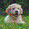
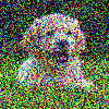
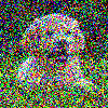

Noise added incrementally to a randomly sampled image \(X_0\) to achieve a noisy image \(X_t\). This is a high dimensional example, inside the high dimensional vector space \(\R^{100 \times 100 \times 3}\). We visualize \(Y_t = X_t / \sqrt{1 + t}\) to keep it in a visual range.
This section introduced stochastic processes, and gave Brownian motion as an example. Luckily don’t need the full tools of stochastic calculus until later, and in the next section will introduce some of the tools for studying the backwards process in diffusion where we just use ordinary differential equations.